Training Overview
In this chapter we provide a cursory overview of RLHF training, before getting into the specifics later in the book. RLHF, while optimizing a simple loss function, involves training multiple, different AI models in sequence and then linking them together in a complex, online optimization.
Here, we introduce the core objective of RLHF, which is optimizing a proxy reward for human preferences with a distance-based regularizer (along with showing how it relates to classical RL problems). Then we showcase canonical recipes which use RLHF to create leading models to show how RLHF fits in with the rest of post-training methods. These example recipes will serve as references for later in the book, where we describe different optimization choices you have when doing RLHF, and we will point back to how different key models used different steps in training.
Problem Formulation
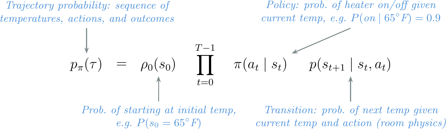
The optimization of reinforcement learning from human feedback (RLHF) builds on top of the standard RL setup. In RL, an agent takes actions \(a_t\) sampled from a policy \(\pi(a_t\mid s_t)\) given the state of the environment \(s_t\) to maximize reward \(r(s_t,a_t)\) [1]. A policy is a function that maps each state to a probability distribution over actions. The early policies that evolved into modern literature on RLHF were in what is called deep reinforcement learning – when a neural network is used to learn said function. Traditionally, the environment evolves according to transition (dynamics) \(p(s_{t+1}\mid s_t, a_t)\) with an initial state distribution \(\rho_0(s_0)\). Together, the policy and dynamics induce a trajectory distribution:
\[p_{\pi}(\tau)=\rho_0(s_0)\prod_{t=0}^{T-1}\pi(a_t\mid s_t)\,p(s_{t+1}\mid s_t,a_t).\qquad{(1)}\]
Across a finite episode with horizon \(T\), the goal of an RL agent is to solve the following optimization, where \(\gamma\) is a discount factor from 0 to 1 that balances the desirability of near-term versus future rewards:
\[\max_\pi \; \mathbb{E}_{\tau \sim p_{\pi}} \left[ \sum_{t=0}^{T-1} \gamma^t r(s_t, a_t) \right],\qquad{(2)}\]
The expected return for a given policy is often denoted \(J(\pi)\), with the optimal value written \(J^* = \max_\pi J(\pi)\).
For continuing tasks, one often takes \(T\to\infty\) and relies on discounting (\(\gamma<1\)) to keep the objective well-defined. Multiple methods for optimizing this expression are discussed in Chapter 6.
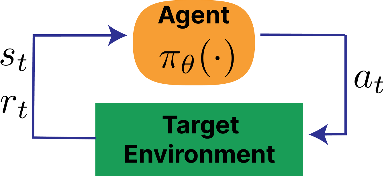
A standard illustration of the RL loop is shown in fig. 1 and (compare this to the RLHF loop in fig. 4).
A Simple Example: The Thermostat
To build a basic intuition for what RL does, consider a thermostat trying to keep a room at a target temperature of 70\(^\circ\)F. In RL, the agent starts with no knowledge of the task and must discover a good policy through trial and error. The thermostat example has the following components (see fig. 2 for how each maps to the trajectory distribution in eq. 1):
- State (\(s_t\)): the current room temperature, e.g. 65\(^\circ\)F.
- Action (\(a_t\)): turn the heater on or off.
- Reward (\(r\)): +1 when the temperature is within 2\(^\circ\) of the target, 0 otherwise.
- Policy (\(\pi\)): the rule that decides whether to turn the heater on or off given the current temperature. An example policy, which may not be optimal depending on the exact transition dynamics of the environment:
\[\pi(a_t = \text{on} \mid s_t) = \begin{cases} 1 & \text{if } s_t < 70^{\circ}\text{F} \\ 0 & \text{otherwise} \end{cases}\qquad{(3)}\]
- Transition: the room warms when the heater is on and cools when it is off. The agent influences these dynamics through its actions, but the underlying physics – how fast the room heats or cools – are outside its control.
Initially, the thermostat’s policy is essentially random – it flips the heater on and off with no regard for the current temperature, and the room swings wildly. Over many episodes of trial and error, the agent discovers that turning the heater on when the room is cold and off when it is warm leads to more reward, and gradually converges on a sensible policy. This is the core RL loop: observe a state, choose an action, receive a reward, and update the policy to get more reward over time.
Example RL Task: CartPole
For a richer example with continuous dynamics, consider the classic CartPole (inverted pendulum) control task, which appears in many RL textbooks, courses, and even research papers. Where the thermostat had a single state variable and a binary action, CartPole involves four continuous state variables and physics-based transitions – making it a standard benchmark for RL algorithms.
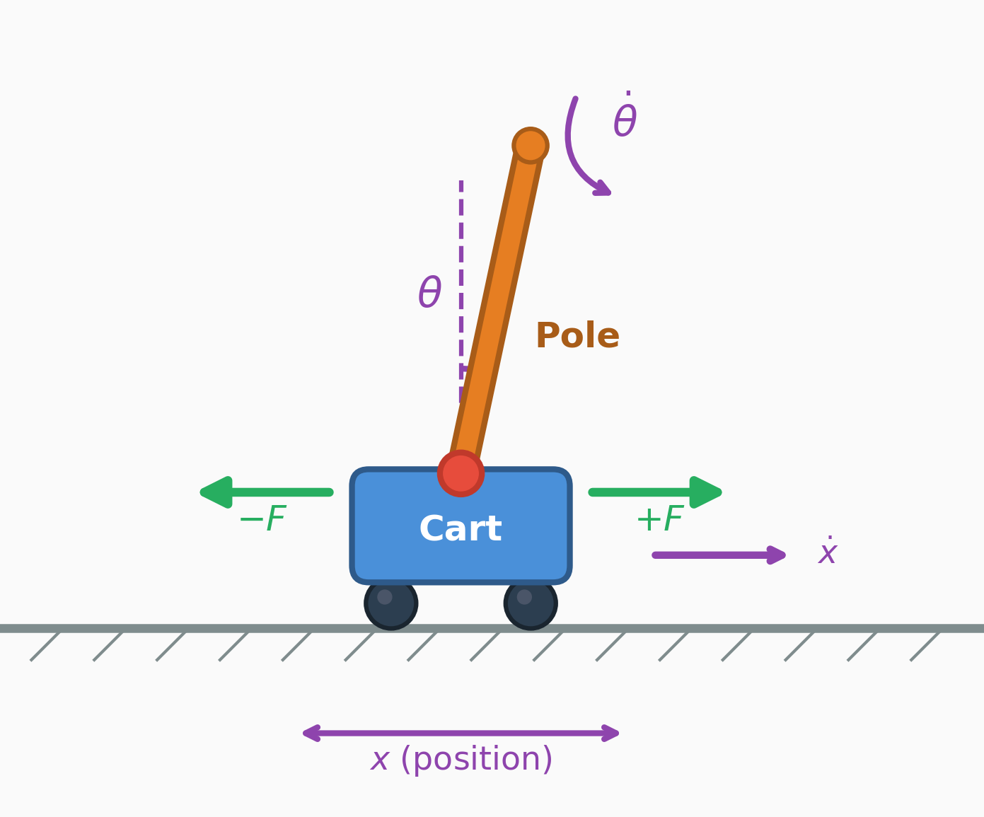
State (\(s_t\)): the cart position/velocity and pole angle/angular velocity,
\[s_t = (x_t,\,\dot{x}_t,\,\theta_t,\,\dot{\theta}_t).\qquad{(4)}\]
Action (\(a_t\)): apply a left/right horizontal force to the cart, e.g. \(a_t \in \{-F, +F\}\).
Reward (\(r\)): a simple reward is \(r_t = 1\) each step the pole remains balanced and the cart stays on the track (e.g. \(|x_t| \le 2.4\) and \(|\theta_t| \le 12^\circ\)), and the episode terminates when either bound is violated.
Dynamics / transition (\(p(s_{t+1}\mid s_t,a_t)\)): in many environments the dynamics are deterministic (so \(p\) is a point mass) and can be written as \(s_{t+1} = f(s_t,a_t)\) via Euler integration with step size \(\Delta t\). A standard simplified CartPole update uses constants cart mass \(m_c\), pole mass \(m_p\), pole half-length \(l\), and gravity \(g\):
\[\text{temp} = \frac{a_t + m_p l\,\dot{\theta}_t^2\sin\theta_t}{m_c + m_p}\qquad{(5)}\]
\[\ddot{\theta}_t = \frac{g\sin\theta_t - \cos\theta_t\,\text{temp}}{l\left(\tfrac{4}{3} - \frac{m_p\cos^2\theta_t}{m_c + m_p}\right)}\qquad{(6)}\]
\[\ddot{x}_t = \text{temp} - \frac{m_p l\,\ddot{\theta}_t\cos\theta_t}{m_c + m_p}\qquad{(7)}\]
\[x_{t+1}=x_t+\Delta t\,\dot{x}_t,\quad \dot{x}_{t+1}=\dot{x}_t+\Delta t\,\ddot{x}_t,\qquad{(8)}\] \[\theta_{t+1}=\theta_t+\Delta t\,\dot{\theta}_t,\quad \dot{\theta}_{t+1}=\dot{\theta}_t+\Delta t\,\ddot{\theta}_t.\qquad{(9)}\]
This is a concrete instance of the general setup above: the policy chooses \(a_t\), the transition function advances the state, and the reward is accumulated over the episode.
Manipulating the Standard RL Setup
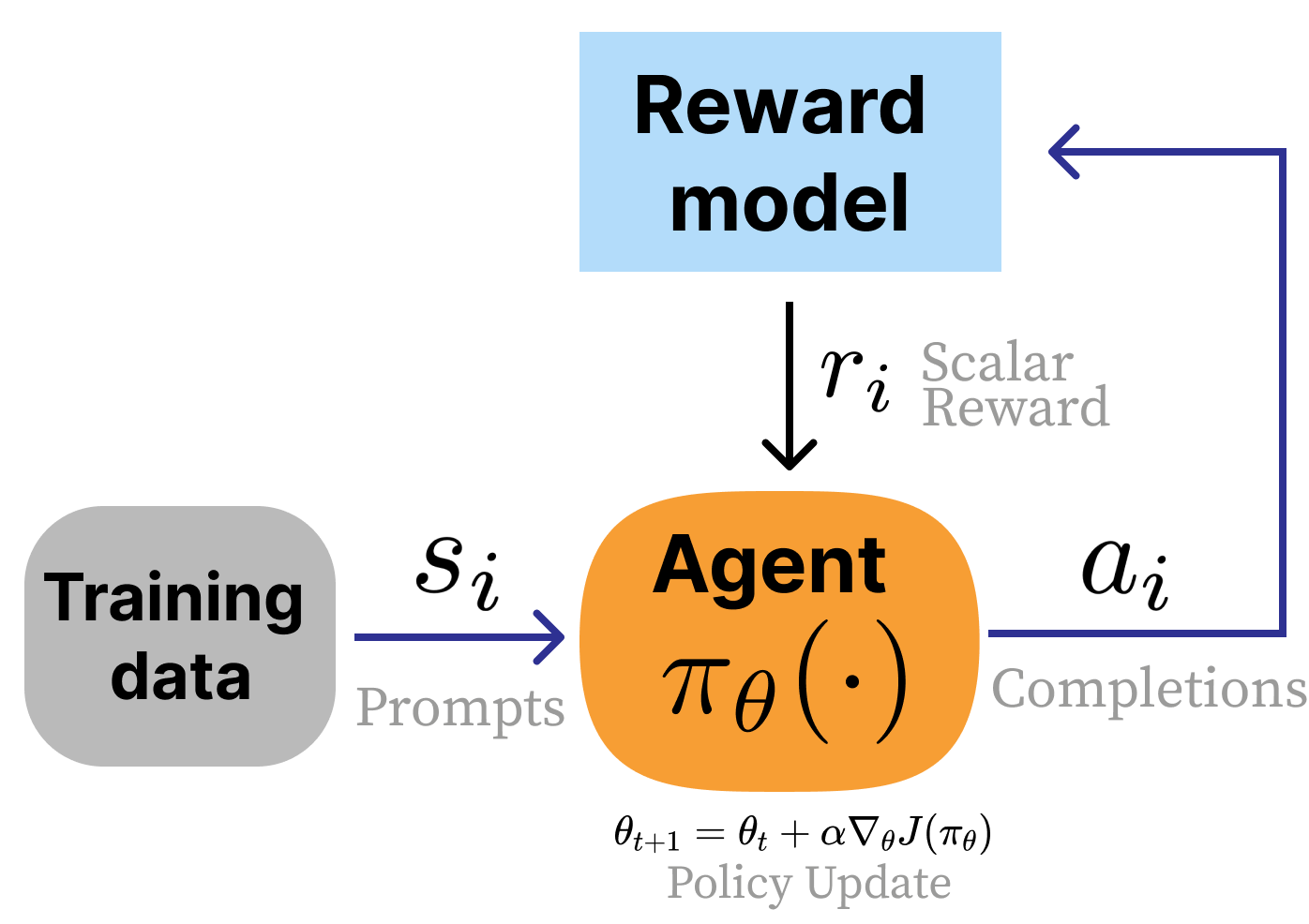
The RL formulation for RLHF is seen as a less open-ended problem, where a few key pieces of RL are set to specific definitions in order to accommodate language models. There are multiple core changes from the standard RL setup to that of RLHF: Table tbl. 1 summarizes these differences between standard RL and the RLHF setup used for language models.
- Switching from a reward function to a reward model. In RLHF, a learned model of human preferences, \(r_\theta(s_t, a_t)\) (or any other classification model) is used instead of an environmental reward function. This gives the designer a substantial increase in the flexibility of the approach and control over the final results, but at the cost of implementation complexity. In standard RL, the reward is seen as a static piece of the environment that cannot be changed or manipulated by the person designing the learning agent.
- No state transitions exist. In RLHF, the initial states for the domain are prompts sampled from a training dataset and the “action” is the completion to said prompt. During standard practices, this action does not impact the next state and is only scored by the reward model.
- Response-level rewards and no discounting. Often referred to as a bandit problem, RLHF attribution of reward is done for an entire sequence of actions, composed of multiple generated tokens, rather than in a fine-grained manner. To help the RL algorithms for RLHF see every token as part of the same action, implementations usually use a discount factor of \(\gamma = 1\) (no discounting), unlike standard RL where \(\gamma < 1\) balances short-term and long-term reward across many sequential decisions.
| Aspect | Standard RL | RLHF (language models) |
|---|---|---|
| Reward signal | Environment reward function \(r(s_t,a_t)\) | Learned reward / preference model \(r_\theta(x,y)\) (prompt \(x\), completion \(y\)) |
| State transition | Yes: dynamics \(p(s_{t+1}\mid s_t,a_t)\) | Typically no: prompts \(x\) sampled from a dataset; the completion does not define the next prompt |
| Action | Single environment action \(a_t\) | A completion \(y\) (a sequence of tokens) sampled from \(\pi_\theta(\cdot\mid x)\) |
| Reward granularity | Often per-step / fine-grained | Usually response-level (bandit-style) over the full completion, usually no discounting (\(\gamma = 1\)) |
| Horizon | Multi-step episode (\(T>1\)) | Often single-step (\(T=1\)), though multi-turn can be modeled as longer-horizon |
Given the single-turn nature of the problem, the optimization can be re-written without the time horizon and discount factor (and with an explicit reward model): \[\max_\pi \; \mathbb{E}_{\tau \sim \pi} \left[r_\theta(s_t, a_t) \right].\qquad{(10)}\]
In many ways, the result is that while RLHF is heavily inspired by RL optimizers and problem formulations, the actual implementation is very distinct from traditional RL.
Fine-tuning and Regularization
In traditional RL problems, the agent must learn from a randomly initialized policy, but with RLHF, we start from a strong pretrained base model with many initial capabilities. This strong prior for RLHF induces a need to prevent the optimization from drifting too far from the initial policy. In order to succeed in a fine-tuning regime, RLHF techniques employ multiple types of regularization to control the optimization. The goal is to allow the reward maximization to still occur without the model succumbing to over-optimization, as discussed in Chapter 14. The most common change to the optimization function is to add a distance penalty on the difference between the current RLHF policy and the starting point of the optimization:
\[\max_\pi \; \mathbb{E}_{\tau \sim \pi} \left[r_\theta(s_t, a_t)\right] - \beta \mathcal{D}_{\text{KL}}(\pi(\cdot|s_t) \| \pi_{\text{ref}}(\cdot|s_t)).\qquad{(11)}\]
Within this formulation, a lot of study into RLHF training goes into understanding how to spend a certain “KL budget” as measured by a distance from the initial model. For more details, see Chapter 15 on Regularization.
Optimization Tools
In this book, we detail many popular techniques for solving this optimization problem. The popular tools of post-training include:
- Reward modeling (Chapter 5): Where a model is trained to capture the signal from collected preference data and can then output a scalar reward indicating the quality of future text.
- Instruction fine-tuning (Chapter 4): A prerequisite to RLHF where models are taught the question-answer format used in the majority of language modeling interactions today by imitating preselected examples.
- Rejection sampling (Chapter 9): The most basic RLHF technique where candidate completions for instruction fine-tuning are filtered by a reward model imitating human preferences.
- Policy gradients (Chapter 6): The reinforcement learning algorithms used in the seminal examples of RLHF to update parameters of a language model with respect to the signal from a reward model.
- Direct alignment algorithms (Chapter 8): Algorithms that directly optimize a policy from pairwise preference data, rather than learning an intermediate reward model to then optimize later.
Modern RLHF-trained models always utilize instruction fine-tuning followed by a mixture of the other optimization options.
Canonical Training Recipes
Over time various models have been identified as canonical recipes for RLHF specifically or post-training generally. These recipes reflect data practices and model abilities at the time. As the recipes age, training models with the same characteristics becomes easier and requires less data. There is a general trend of post-training involving more optimization steps with more training algorithms across more diverse training datasets and evaluations.
InstructGPT
Around the time ChatGPT first came out, the widely accepted (“canonical”) method for post-training an LM had three major steps, with RLHF being the central piece [2] [3] [4]. The three steps taken on top of a “base” language model (the next-token prediction model trained on large-scale web text) are summarized below in fig. 5:
- Instruction tuning on ~10K examples: This teaches the model to follow the question-answer format and teaches some basic skills from primarily human-written data.
- Training a reward model on ~100K pairwise prompts: This model is trained from the instruction-tuned checkpoint and captures the diverse values one wishes to model in their final training. The reward model is the optimization target for RLHF.
- Training the instruction-tuned model with RLHF on another ~100K prompts: The model is optimized against the reward model with a set of prompts that the model generates responses to before receiving ratings.
Once RLHF was done, the model was ready to be deployed to users. This recipe is the foundation of modern RLHF, but recipes have evolved substantially to include more stages and more data.
Tülu 3
Modern versions of post-training involve many, many more model versions and training stages (i.e. well more than the 5 RLHF steps documented for Llama 2 [5]). An example is shown below in fig. 6 where the model undergoes numerous training iterations before convergence.
The most complex models trained in this era and onwards have not released full details of their training process. Leading models such as ChatGPT or Claude circa 2025 involve many, iterative rounds of training. This can even include techniques that train specialized models and then merge the weights together to get a final model capable on many subtasks [6] (e.g. Cohere’s Command A [7]).
A fully open example of this multi-stage approach to post-training where RLHF plays a major role is Tülu 3. The Tülu 3 recipe consists of three stages:
- Instruction tuning on ~1M examples: This primarily synthetic data from a mix of frontier models such as GPT-4o and Llama 3.1 405B teaches the model general instruction following and serves as the foundation of a variety of capabilities such as mathematics or coding.
- On-policy preference data on ~1M preference pairs: This stage substantially boosts the chattiness (e.g. ChatBotArena or AlpacaEval 2) of the model while also improving skills mentioned above in the instruction tuning stage.
- Reinforcement Learning with Verifiable Rewards on ~10K prompts: This stage is a small-scale reinforcement learning run to boost core skills such as mathematics while maintaining overall performance (and is now seen as a precursor to modern reasoning models such as DeepSeek R1).
The recipe has been successfully applied to Llama 3.1 [8], OLMo 2 [9], and SmolLM models [10].
DeepSeek R1
With the rise of reasoning language models, such as OpenAI’s o1, the best practices in post-training evolved again to re-order and redistribute compute across training stages. The clearest documentation of a reasoning model post-training recipe is DeepSeek R1 [11], which has been mirrored by Alibaba’s larger Qwen 3 models (i.e. only the 32B and 225B MoE models) [12] or Xiaomi’s MiMo 7B [13]. The DeepSeek recipe follows:
- “Cold-start” of 100K+ on-policy reasoning samples: This data is sampled from an earlier RL checkpoint, R1-Zero, and heavily filtered to instill a specific reasoning process on the model. DeepSeek uses the term cold-start to describe how RL is learned from little supervised data.
- Large-scale reinforcement learning training: This stage repeatedly covers reasoning problems with the model, running RLVR “until convergence” on a variety of benchmarks.
- Rejection sampling on 3/4 reasoning problems and 1/4 general queries to start the transition to a general-purpose model.
- Mixed reinforcement learning training on reasoning problems (verifiable rewards) with general preference tuning reward models to polish the model.
As above, there are evolutions of the recipe, particularly with steps 3 and 4 to finalize the model before exposing it to users. Many models start with tailored instruction datasets with chain-of-thought sequences that are heavily filtered and polished from existing models, providing a fast step to strong behaviors with SFT alone before moving onto RL [14].