Regularization
Throughout the RLHF optimization, many regularization steps are used to prevent over-optimization of the reward model. Over-optimization in these contexts looks like models that output nonsensical text. Some examples of optimization “off the rails” are that models can output followable math reasoning with extremely incorrect answers, repeated text, switching languages, or excessive special characters. This chapter covers the different methods that’re used to control the optimization of models.
The most popular variant, used in most RLHF implementations at the time of writing, is a KL distance from the current policy to a reference policy across generated samples. “KL distance” is a colloquial term for expressing the optimization distance within the training process, even though KL divergence—the underlying mathematical method for measuring the separation of two probability distributions—does not satisfy the formal properties required to be a true distance metric (it is simply easier to call the number a distance than a numeric measure of distributional difference). Many other regularization techniques have emerged in the literature to then disappear in the next model iteration in that line of research. That is to say that regularization outside the core KL distance from generations is often used to stabilize experimental setups that can then be simplified in the next generation. Still, it is important to understand tools to constrain optimization in RLHF.
Throughout this chapter, we use \(x\) to denote prompts and \(y\) to denote completions. This notation is common in the language model literature, where methods operate on full prompt-completion pairs rather than individual tokens.
The general formulation, when used in an RLHF framework with a reward model, \(r_\theta\) is as follows:
\[ r = r_\theta - \lambda r_{\text{reg.}} \qquad{(1)}\]
With the reference implementation being:
\[ r = r_\theta - \lambda_{\text{KL}} \mathcal{D}_{\text{KL}} \left( \pi_{\text{RL}}(y \mid x) \, \| \, \pi_{\text{ref}}(y \mid x) \right) \qquad{(2)}\]
KL Divergences in RL Optimization
For mathematical definitions, see Appendix A on Definitions. Recall that a KL divergence measure of probability difference is defined as follows:
\[ \mathcal{D}_{\text{KL}}(P || Q) = \sum_{x \in \mathcal{X}} P(x) \log \left(\frac{P(x)}{Q(x)}\right) \qquad{(3)}\]
In RLHF, the two distributions of interest are often the distribution of the new model version, say \(P(x)\), and a distribution of the reference policy, say \(Q(x)\). Different optimizers use different KL directions. Throughout this book, the most common “KL Penalty” that is used is called the reverse KL to the reference policy. In practice, this reduces to a Monte Carlo estimate that samples tokens from the RL model and computes probabilities from the reference model. Intuitively, this reverse KL has a numerical property that applies a large penalty when the new model, \(P\) or \(\pi_{\text{RL}}\), puts substantial probability mass where the original reference model assigns low probability.
The other KL direction is still often used in ML, e.g. in the internal trust region calculation of some RL algorithms. This penalty intuitively penalizes the new model when its update does not apply probability to a high-likelihood region in \(Q\) or \(\pi_{\text{ref}}\). This is closer to an objective used for distillation or behavioral cloning.
Reference Model to Generations
KL penalties are most commonly implemented by comparing the distance between the generated tokens during training to a static reference model. The intuition is that the model you’re training from has a style that you would like to stay close to. This reference model is most often the instruction tuned model, but can also be a previous RL checkpoint. With simple substitution, the model we are sampling from becomes \(\pi_{\text{RL}}(x)\) and \(\pi_{\text{ref}}(x)\), shown above in eq. 2 (often \(P\), and \(Q\), in standard definitions, when applied for RL KL penalties). Such a KL divergence penalty was first applied to dialogue agents well before the popularity of large language models [1], yet KL control was quickly established as a core technique for fine-tuning pretrained models [2].
Implementation Example
In practice, the implementation of KL divergence is often approximated [3], making the implementation far simpler. With the above definition, the summation of KL can be converted to an expectation when sampling directly from the distribution \(P(x)\). In this case, the distribution \(P(x)\) is the generative distribution of the model currently being trained (i.e. not the reference model). Then, the computation for KL divergence changes to the following:
\[ \mathcal{D}_{\text{KL}}(P \,||\, Q) = \mathbb{E}_{x \sim P} \left[ \log P(x) - \log Q(x) \right]. \qquad{(4)}\]
This mode is far simpler to implement, particularly when dealing directly with log probabilities used frequently in language model training.
# Step 1: sample (or otherwise generate) a sequence from your policy
generated_tokens = model.generate(inputs)

# Step 2: score that generated sequence under both models
#    for autoregressive LMs, you usually do:
#      inputs_for_scoring = generated_tokens[:, :-1]
#      labels           = generated_tokens[:, 1:]
logits       = model.forward(generated_tokens[:, :-1]).logits
ref_logits   = ref_model.forward(generated_tokens[:, :-1]).logits

# convert to log-probs, then align labels to index into the logits
logprobs     = F.log_softmax(logits, dim=-1)
ref_logprobs = F.log_softmax(ref_logits, dim=-1)

# gather the log-probs of the actual next tokens
token_logprobs     = logprobs.gather(-1, generated_tokens[:, 1:].unsqueeze(-1)).squeeze(-1)
ref_token_logprobs = ref_logprobs.gather(-1, generated_tokens[:, 1:].unsqueeze(-1)).squeeze(-1)

# now you can sum (or average) those to get the sequence log-prob,
# and compute KL:
seq_logprob     = token_logprobs.sum(dim=-1)
ref_seq_logprob = ref_token_logprobs.sum(dim=-1)

kl_approx = seq_logprob - ref_seq_logprob
kl_full   = F.kl_div(ref_logprobs, logprobs, reduction='batchmean')
Some example implementations include TRL and Hamish Ivison’s Jax Code.
Pretraining Gradients
Another way of viewing regularization is that you may have a dataset that you want the model to remain close to, as done in InstructGPT [4] “in order to fix the performance regressions on public NLP datasets”. To implement this, they modify the training objective for RLHF. Taking eq. 1, we can transform this into an objective function to optimize by sampling from the RL policy model, completions \(y\) from prompts \(x\) in the RL dataset used for RLHF, which yields: \[ J(\theta) = \mathbb{E}_{(x,y) \sim \mathcal{D}_{\pi_{\text{RL},\theta}}} \left[ r_{\theta}(y \mid x) - \lambda r_{\text{reg.}} \right] \qquad{(5)}\]
Then, we can add an additional reward for higher probabilities on the standard autoregressive next-token prediction loss used at pretraining, over a set of documents sampled from the pretraining corpus (or another dataset) to maintain textual coherence:
\[ J(\theta) = \mathbb{E}_{(x,y) \sim \mathcal{D}_{\pi_{\text{RL},\theta}}} \left[ r_{\theta}(y \mid x) - \lambda r_{\text{reg.}} \right] + \gamma \mathbb{E}_{x \sim \mathcal{D}_{\text{pretrain}}} \left[ \log(\pi_{\text{RL},\theta}(x)) \right] \qquad{(6)}\]
Recent work proposed using a negative log-likelihood term to balance the optimization of Direct Preference Optimization (DPO) [5]. Given the pairwise nature of the DPO loss, the same loss modification can be made to reward model training, constraining the model to predict accurate text (rumors from laboratories that did not publish the work).
The optimization follows as a modification to DPO. \[\mathcal{L}_{\text{DPO+NLL}} = \mathcal{L}_{\text{DPO}}(c_i^w, y_i^w, c_i^l, y_i^l \mid x_i) + \alpha \mathcal{L}_{\text{NLL}}(c_i^w, y_i^w \mid x_i) \qquad{(7)}\]
\[ = -\log \sigma \left( \beta \log \frac{P_\theta(c_i^w, y_i^w \mid x_i)}{P_{\text{ref.}}(c_i^w, y_i^w \mid x_i)} - \beta \log \frac{P_\theta(c_i^l, y_i^l \mid x_i)}{P_{\text{ref.}}(c_i^l, y_i^l \mid x_i)} \right) - \alpha \frac{\log P_\theta(c_i^w, y_i^w \mid x_i)}{|c_i^w| + |y_i^w|}, \qquad{(8)}\]
where \(P_{\theta}\) is the trainable policy model, \(P_{\text{ref.}}\) is a fixed reference model (often the SFT checkpoint), and \((c_i^w, y_i^w)\) and \((c_i^l, y_i^l)\) denote the winning and losing completions for prompt \(x_i\). The first term is the standard DPO logistic loss: it increases the margin between the win and loss using the difference of log-likelihood ratios, \(\log \tfrac{P_{\theta}}{P_{\text{ref.}}}\), and \(\beta\) controls how strongly this preference signal pulls away from the reference. The second term is a length-normalized negative log-likelihood penalty on the winning completion, weighted by \(\alpha\), which helps keep the preferred text high-likelihood in an absolute language modeling sense rather than only relatively better than the rejected sample.
Margin-based Regularization
Controlling the optimization is less well defined in other parts of the RLHF stack. Most reward models have no regularization beyond the standard contrastive loss function. Direct Alignment Algorithms handle regularization to KL divergences differently, through the \(\beta\) parameter (see the chapter on Direct Alignment).
Llama 2 proposed a margin loss for reward model training [6]:
\[ \mathcal{L}(\theta) = - \log \left( \sigma \left( r_{\theta}(y_c \mid x) - r_{\theta}(y_r \mid x) - m(y_c, y_r) \right) \right) \qquad{(9)}\]
where \(m(y_c, y_r)\) is the margin between two datapoints \(y_c\) and \(y_r\) representing numerical difference in delta between the ratings of two annotators. This is either achieved by having annotators rate the outputs on a numerical scale or by using a quantified ranking method, such as Likert scales.
Reward margins have been used heavily in the direct alignment literature, such as Reward weighted DPO, ‘’Reward-aware Preference Optimization’’ (RPO), which integrates reward model scores into the update rule following a DPO loss [7], or REBEL [8] that has a reward delta weighting in a regression-loss formulation.
Implicit Regularization
The preceding sections describe explicit regularization: KL penalties, pretraining gradients, and margin losses that practitioners deliberately add to the training objective. A growing body of empirical work reveals that RL-based post-training also provides implicit regularization — a built-in resistance to memorization and catastrophic forgetting that emerges from the structure of on-policy optimization itself, even without any explicit KL penalty or replay buffer.
SFT Memorizes, RL Generalizes
A core question facing the post-training community has been: When training on a single task, does the model learn a generalizable rule that transfers to unseen variants, or does it memorize the surface patterns of the training distribution? [9] answer this question with a controlled empirical study that directly isolates the effect of the post-training method — SFT versus RL — on out-of-distribution (OOD) generalization. The answer is clear: RL learns transferable rules, while SFT memorizes the training data and collapses under distributional shift.
The study uses two environments with built-in rule variations:
GeneralPoints is an arithmetic card game where the model receives four playing cards and must combine their numerical values with operators (+, -, *, /) to reach a target number (24 by default). The OOD test changes how face cards are scored: training uses one rule (Jack, Queen, and King all count as 10), evaluation uses another (Jack = 11, Queen = 12, King = 13).
V-IRL is a real-world visual navigation task where models follow linguistic instructions to traverse a route through city streets, recognizing landmarks along the way. The OOD shift switches the action space from absolute directions (north, east) to relative directions (left, right).
Across all task variants, RL consistently improves OOD performance as training compute scales up, while SFT consistently degrades OOD performance despite improving in-distribution. The magnitude of divergence is striking: on V-IRL with language-only inputs, where the OOD shift is from absolute to relative directional coordinates, RL improves OOD per-step accuracy from 80.8% to 91.8%, while SFT collapses from 80.8% to 1.3%. The SFT model goes further than failing to generalize: it destroys the spatial reasoning the base model already had, collapsing to a lookup table from instruction phrases to absolute directions.
Retaining by Doing: On-Policy Data Mitigates Forgetting
The previous section showed that RL generalizes where SFT memorizes on a single task. [10] ask the complementary question: when training sequentially on multiple tasks, does the model retain what it already knew? They find that RL achieves comparable or higher gains on target tasks while forgetting substantially less than SFT, and trace this advantage to a fundamental difference in what the two objectives optimize.
To understand why the two methods behave so differently, we can view their objectives through the lens of KL divergence, which can be expressed in two directions:
- Forward KL: \(\text{KL}(P \| Q) = \mathbb{E}_{x \sim P}[\log P(x) - \log Q(x)]\)
- Reverse KL: \(\text{KL}(Q \| P) = \mathbb{E}_{x \sim Q}[\log Q(x) - \log P(x)]\)
where \(P\) is the target distribution and \(Q\) is the distribution we are modeling with parameters \(\theta\). The key difference is which distribution we sample from: forward KL samples from the target (or optimal) distribution \(P\), whereas reverse KL samples from our policy \(Q\). In the derivations below, \(P\) corresponds to the target \(\pi_\star\) (the training data distribution when analyzing SFT, or the reward-optimal policy when analyzing RL) and \(Q\) to the learned policy \(\pi_\theta\). SFT places the target first — \(\text{KL}(\pi_\star \| \pi_\theta)\) — while RL flips the order — \(\text{KL}(\pi_\theta \| \pi_\star)\) — changing which distribution we sample from.
SFT \(\approx\) Forward KL. Let \(\pi_\star\) be the target distribution for our dataset. Then, the forward KL divergence is:
\[ \begin{aligned} \text{KL}(\pi_\star \| \pi_\theta) &= \mathbb{E}_{(x,y) \sim \mathcal{D}} \left[ \log \pi_\star(y \mid x) - \log \pi_\theta(y \mid x) \right] \\ &= \mathbb{E}_{(x,y) \sim \mathcal{D}} \left[ \log \pi_\star(y \mid x) \right] - \mathbb{E}_{(x,y) \sim \mathcal{D}} \left[ \log \pi_\theta(y \mid x) \right] \\ &= \underbrace{-H(\pi_\star)}_\text{const} + \mathcal{L}_\text{SFT}(\theta) \\ &\propto \mathcal{L}_\text{SFT}(\theta) \end{aligned} \qquad{(10)}\]
Since \(H(\pi_\star)\) is constant with respect to \(\theta\), minimizing the SFT loss is exactly equivalent to minimizing the forward KL divergence \(\text{KL}(\pi_\star \| \pi_\theta)\).
RL \(\approx\) Reverse KL. Let us start with the standard KL-regularized RL objective:
\[ \max_\pi \; \mathcal{J}_\text{RL}(\theta) = \mathbb{E}_{x \sim \mathcal{D},\, y \sim \pi(\cdot \mid x)} \left[ r(x, y) \right] - \beta \cdot \text{KL}\!\left(\pi(\cdot \mid x) \| \pi_\text{ref}(\cdot \mid x)\right) \qquad{(11)}\]
Pulling out \(-\beta\) converts maximization to minimization:
\[ = \min_\pi \; \mathbb{E}_{x \sim \mathcal{D},\, y \sim \pi(\cdot \mid x)} \left[ \log \frac{\pi(y \mid x)}{\pi_\text{ref}(y \mid x)} - \frac{1}{\beta} r(x, y) \right] \qquad{(12)}\]
Introducing a partition function \(Z(x) = \sum_y \pi_\text{ref}(y \mid x) \exp\!\left(\frac{1}{\beta} r(x,y)\right)\) to normalize the reward-tilted reference into a valid distribution, and adding and subtracting \(\log Z(x)\), the inner expectation becomes a KL divergence:
\[ = \min_\pi \; \mathbb{E}_{x \sim \mathcal{D}} \left[ \text{KL}\!\left(\pi(\cdot \mid x) \;\middle\|\; \frac{1}{Z(x)} \pi_\text{ref}(\cdot \mid x) \exp\!\left(\tfrac{1}{\beta} r(x,y)\right) \right) - \log Z(x) \right] \qquad{(13)}\]
Since \(\log Z(x)\) does not depend on \(\pi\), the KL is minimized at zero when \(\pi\) equals the reward-tilted distribution. The optimal policy under reward \(r(x,y)\) is therefore:
\[ \pi_\star(y \mid x) = \frac{1}{Z(x)} \pi_\text{ref}(y \mid x) \exp\!\left(\frac{1}{\beta} r(x,y)\right) \qquad{(14)}\]
Now we can show the connection to reverse KL directly. Expanding \(\text{KL}(\pi_\theta \| \pi_\star)\) and substituting \(\log \pi_\star(y \mid x) = \log \pi_\text{ref}(y \mid x) - \log Z(x) + \frac{1}{\beta} r(x, y)\):
\[ \begin{aligned} \text{KL}(\pi_\theta \| \pi_\star) &= \mathbb{E}_{x \sim \mathcal{D},\, y \sim \pi_\theta(\cdot \mid x)} \left[ \log \pi_\theta(y \mid x) - \log \pi_\star(y \mid x) \right] \\ &= \mathbb{E}_{x \sim \mathcal{D},\, y \sim \pi_\theta(\cdot \mid x)} \left[ \log \pi_\theta(y \mid x) - \log \pi_\text{ref}(y \mid x) + \log Z(x) - \frac{1}{\beta} r(x, y) \right] \\ &= - \frac{1}{\beta} \mathbb{E}_{x,y}\!\left[r(x,y)\right] + \text{KL}\!\left(\pi_\theta(\cdot \mid x) \;\middle\|\; \pi_\text{ref}(\cdot \mid x)\right) + \underbrace{\log Z(x)}_\text{const} \\ &\propto - \frac{1}{\beta} \mathbb{E}_{x,y}\!\left[r(x,y)\right] + \text{KL}\!\left(\pi_\theta(\cdot \mid x) \;\middle\|\; \pi_\text{ref}(\cdot \mid x)\right) \\ &= -\frac{1}{\beta} \mathcal{J}_\text{RL}(\theta) \end{aligned} \]
Equivalently, maximizing the RL objective \(\mathcal{J}_\text{RL}(\theta)\) is the same as minimizing the reverse KL divergence \(\text{KL}(\pi_\theta \| \pi_\star)\).
This derivation shows that SFT and RL optimize fundamentally different objectives: SFT minimizes forward KL, RL minimizes reverse KL.
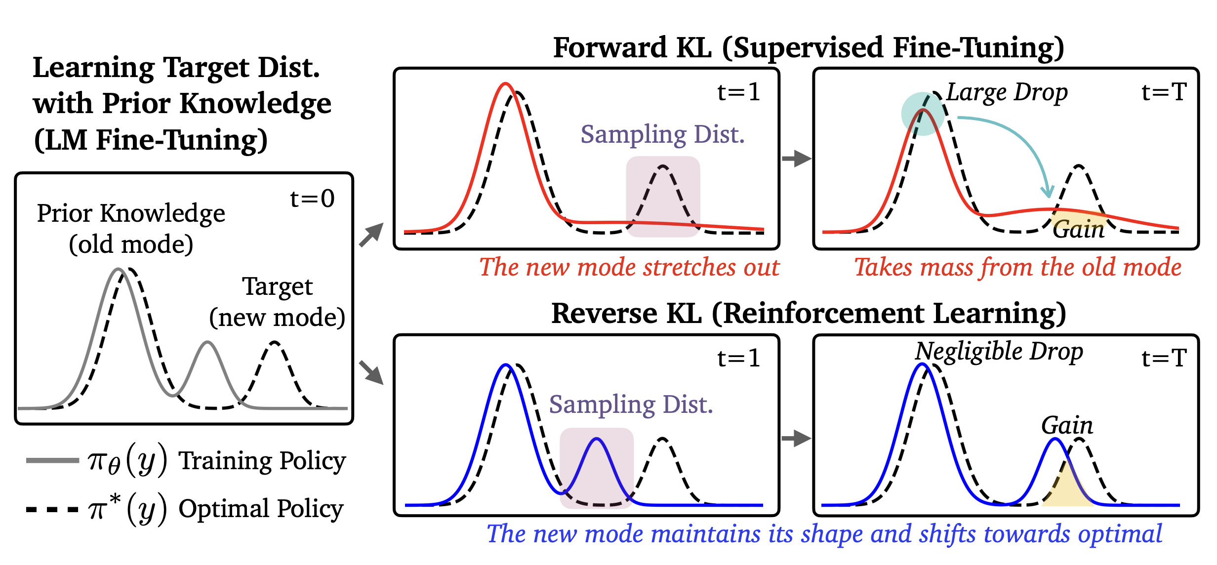
Forward KL penalizes the model whenever the target distribution has mass where the model does not, which forces the model to cover all modes of the target — spreading probability broadly even if it means assigning mass to low-probability regions (mode covering). Reverse KL only penalizes the model in regions where it actually places mass, which allows it to seek a single mode and fit it precisely while ignoring others entirely (mode seeking).
Given this distinction, we might naively expect SFT to forget less than RL: mode-covering forward KL should maintain mass across all modes of the target, preserving old knowledge, while mode-seeking reverse KL could collapse onto a single high-reward mode and abandon others.
However, the opposite holds. This intuition assumes a unimodal policy, but pre-trained LLMs contain multiple modes — and for multimodal distributions, the dynamics flip.
Consider a policy with two modes: an “old” mode representing prior knowledge and a “new” mode for the target task (fig. 1). Forward KL (SFT) must cover both modes of the target distribution, which forces the policy to stretch and redistribute probability mass from the old mode, disrupting its shape and causing forgetting. Reverse KL (RL), by contrast, only needs to place mass on some high-reward region, so it can shift the new mode toward the target without touching the old mode at all, leaving prior knowledge intact.
RL’s mode-seeking behavior — a structural property of reverse KL — preserves the breadth of the model’s prior knowledge and enables better generalization.
To summarize:
SFT (Forward KL): \(\text{KL}(\pi_\star \| \pi_\theta)\) — samples come from the target \(\pi_\star\), a fixed dataset of human-written completions. For each example, we ask: how much probability does our model \(\pi_\theta\) assign to this? The model never generates anything; it learns to imitate. This mode-covering pressure forces the policy to redistribute mass broadly, which can disrupt prior knowledge.
RL (Reverse KL): \(\text{KL}(\pi_\theta \| \pi_\star)\) — samples come from our own policy \(\pi_\theta\). For each completion the model generates, we ask: how close is this to the reward-optimal policy \(\pi_\star\)? Because the model only trains on its own generations, updates stay local to where it already places probability mass — the reward signal tells it which of those generations to reinforce, shifting probability toward \(\pi_\star\) without disturbing the rest of the distribution.
RL’s Razor: Why Online RL Forgets Less
The previous section showed that on-policy sampling drives RL’s forgetting resistance and traced the mechanism to forward-vs-reverse KL dynamics. [11] offer a complementary perspective, again through the lens of KL divergence.
For any given task, there exist many distinct policies which achieve high performance. [11] introduce the RL’s Razor thesis which postulates the following:
Among the many high-reward solutions for a new task, on-policy methods such as RL are inherently biased toward solutions that remain closer to the original policy in KL divergence.
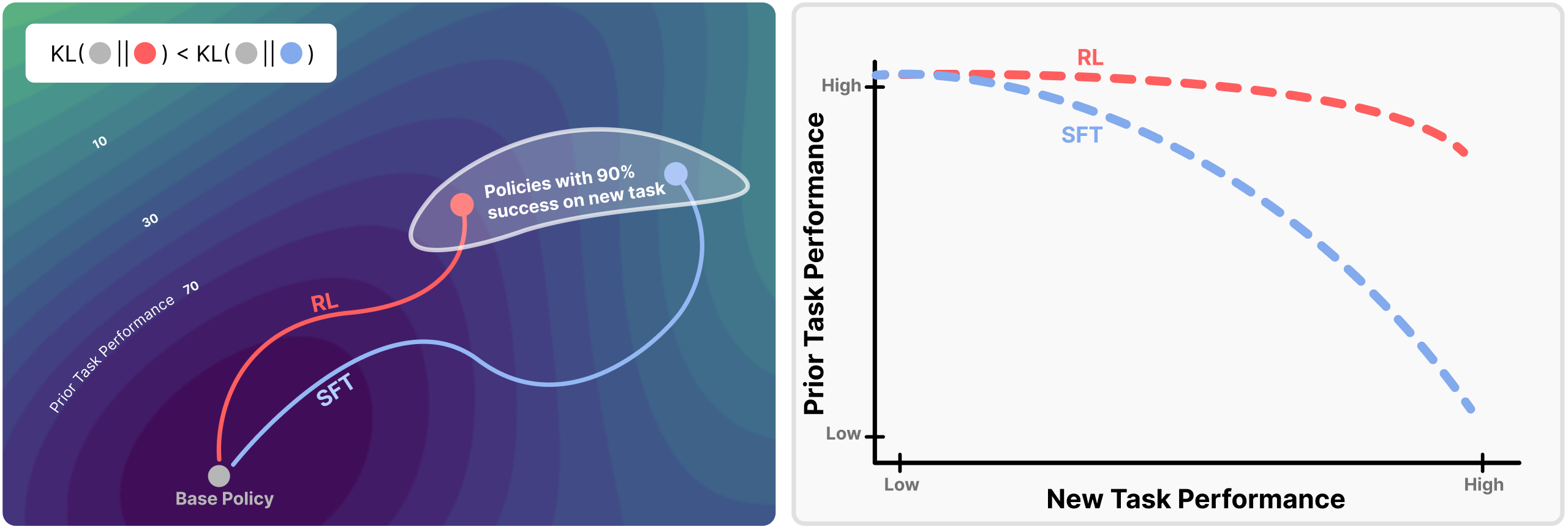
The authors find that forgetting of past tasks is directly proportional to how far the fine-tuned policy drifts from the initial model as measured by the KL divergence:
\[ \text{Forgetting} \approx f\!\left(\mathbb{E}_{x \sim \tau}\!\left[\text{KL}\!\left(\pi_0(\cdot \mid x) \| \pi(\cdot \mid x)\right)\right]\right) \qquad{(15)}\]
Across several training flavors of RL and SFT, the authors empirically demonstrate that forgetting strongly correlates (\(R^2 = 0.96\)) with the KL divergence between the trained and initial policies, as measured using the new task data. The result is highly non-trivial: the KL is measured on the new task’s input distribution, not on held-out data from prior tasks, yet it still predicts the performance drop on past tasks. In practice, this provides us with a powerful instrument for estimating forgetting directly from the drift between the base and trained policies.
To pin down what drives the smaller KL shifts in RL policies, the authors decompose the difference between RL and SFT along two axes — on-policy versus offline data, and whether the objective includes negative gradients (present in RL when samples score below the reward baseline, absent in SFT which only reinforces correct demonstrations) that push probability away from incorrect outputs. Remarkably, they find that on-policy versus offline data fully accounts for the difference in generalization performance, while negative gradients have no discernible effect.
Intuitively, on-policy methods sample outputs the model already assigns non-negligible probability to, so each update is constrained to stay near the current distribution. On the other hand, SFT trains on a fixed external distribution that can lie arbitrarily far from what the model currently produces, and each gradient step pulls toward that distant target regardless of the model’s own beliefs.