Nathan Lambert

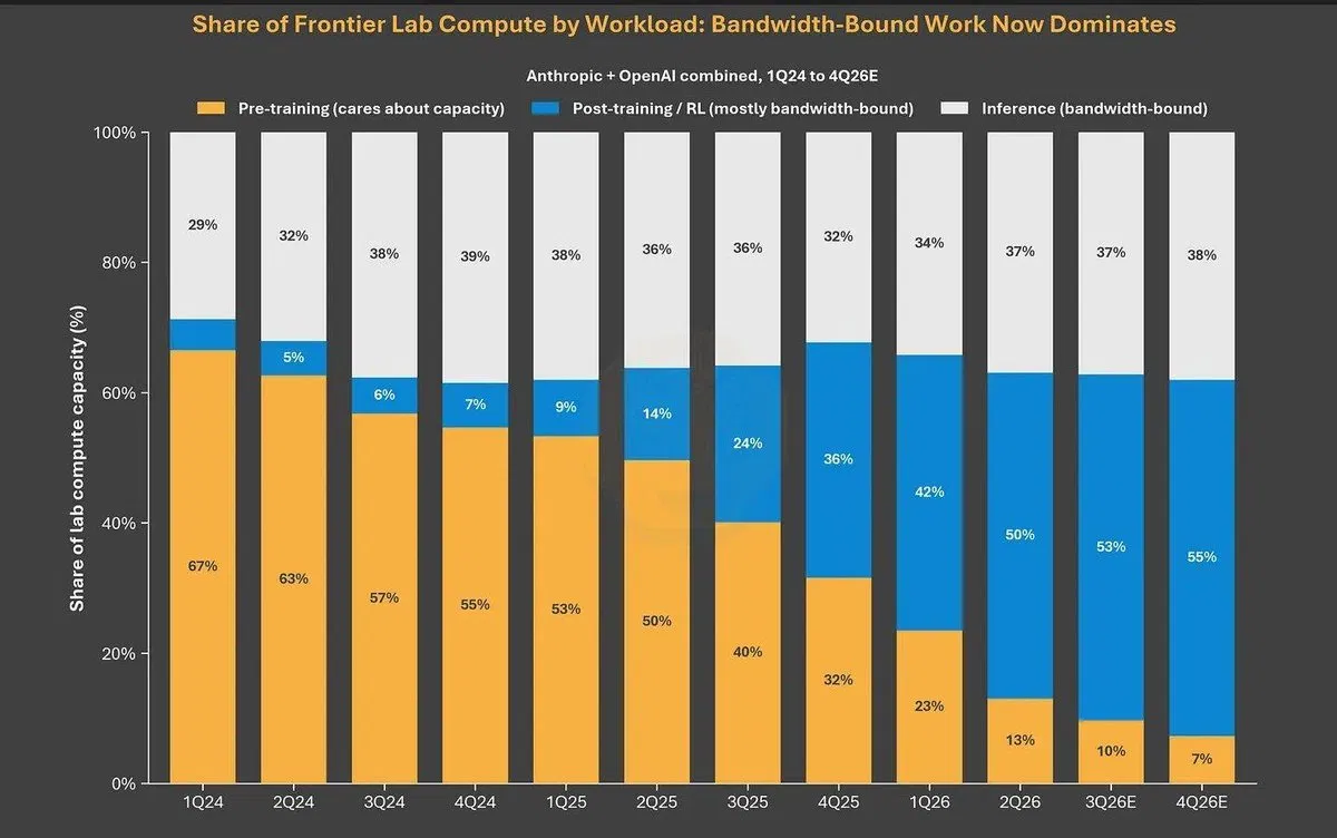
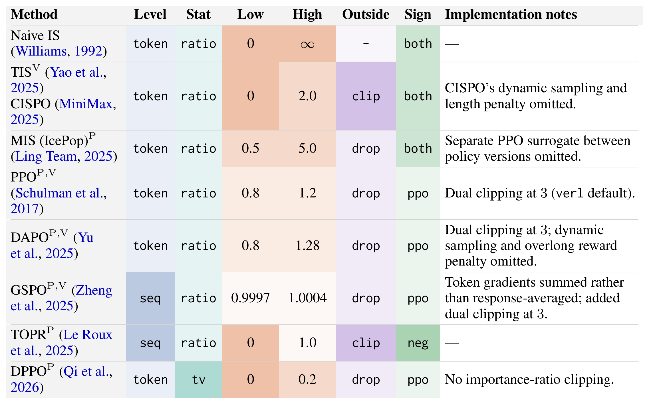
RL compute relative to pretraining compute for the same model, in GPU-hours:
| Model | Pretraining | RL | RL / pretraining |
|---|---|---|---|
| DeepSeek R1 Jan 2025 671B total, 37B active |
2.66M H800 GPU-hours (DeepSeek-AI, 2025) | 0.14M H800 GPU-hours (Guo et al., 2025) | ~5% |
| Beam Oct 2026 501B total, 23B active |
< 4.1M 6,144 GB300s for under 4 weeks | ~7.1M 10.5K GB300s for 4 weeks | > 1.7× |
| Inkling 2 Small Nov 2026 594B total, 17B active |
~0.11M* ~1.5K GPUs for under 3 days | ~0.44M 2,048 GPUs for 9 days | ~4×* |
How RL is approached with LLMs and what the challenges of RL are for frontier models.
RL is mostly an engineering, stability, and throughput problem at the frontier. The learning signal is important, and mostly comes through data engineering (not the focus of this lecture).
How RL is approached with LLMs and what the challenges of RL are for frontier models.
Some examples we include:
| Symbol | Meaning | Book / lectures |
|---|---|---|
| x | Prompt | s |
| a = (a_1, \dots, a_T) | Completion, one token at a time | a |
| v \in \mathcal{V} | Any token in the vocabulary | v |
| p_\theta | Learner: the training framework’s (e.g., FSDP) next-token distribution | \pi_\theta^{\text{learner}} |
| q | Sampler: the inference engine’s (e.g., vLLM) next-token distribution (no gradient updates) | \pi_\theta^{\text{sampler}} |
| f_\theta | Logits, so p_\theta = \text{softmax}(f_\theta) | |
| \boldsymbol{\xi}_v = \nabla_\theta \log p_v | Gradient “score” of token v | \boldsymbol{\xi}_v |
| A | Advantage for the whole completion, e.g., r - b(x) | A |
p_v and q_v are shorthand for the probability of token v at one position, given x and the prefix a_{<t}. CS 4789 uses the same x and a.
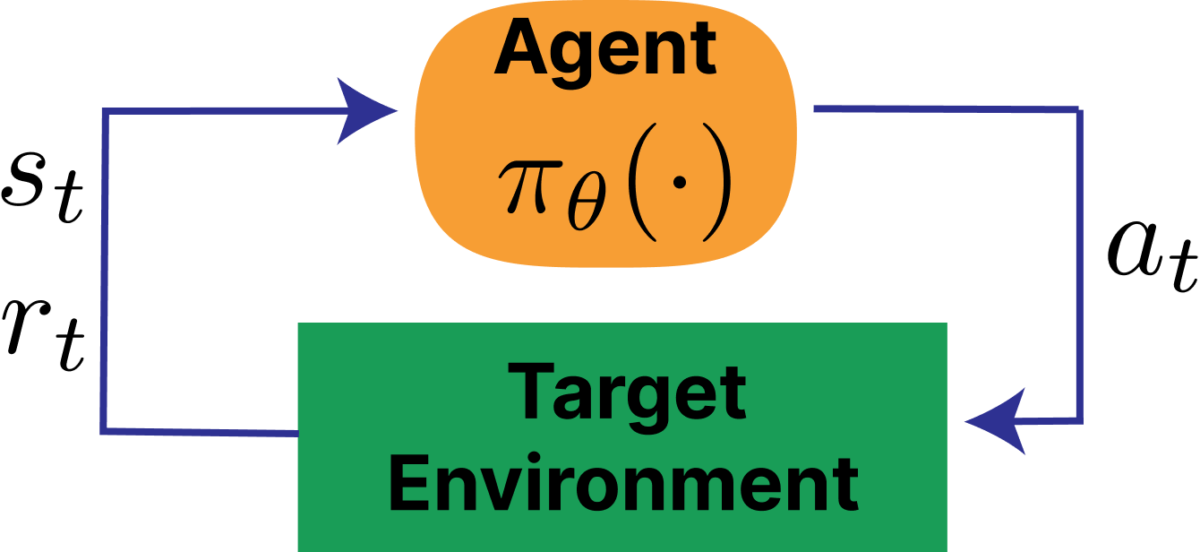
Classical RL: agent in an MDP (\mathcal{S}, \mathcal{A}, P, r, \gamma)

| MDP concept | Language model |
|---|---|
| State s_t | Prompt + tokens generated so far: (x, a_{<t}) |
| Action a_t | Next token a_t |
| Transition | Deterministic-ish: append token to sequence (tokens are sampled probabilistically) |
| Policy \pi_\theta(a_t \mid s_t) | LM next-token distribution |
| Episode | One prompt → completion |
| Terminal reward | RM score, verifier output, judge-scores |
| \gamma | Typically 1.0 (no discounting) |
Two implementation-level views of this MDP: token-level (each token is a separate action, used in PPO with GAE) vs. sequence-level (entire completion is one action, used in REINFORCE/GRPO).
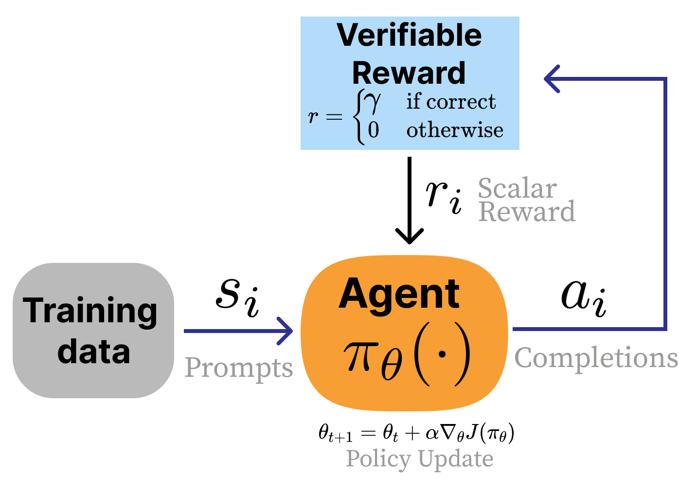
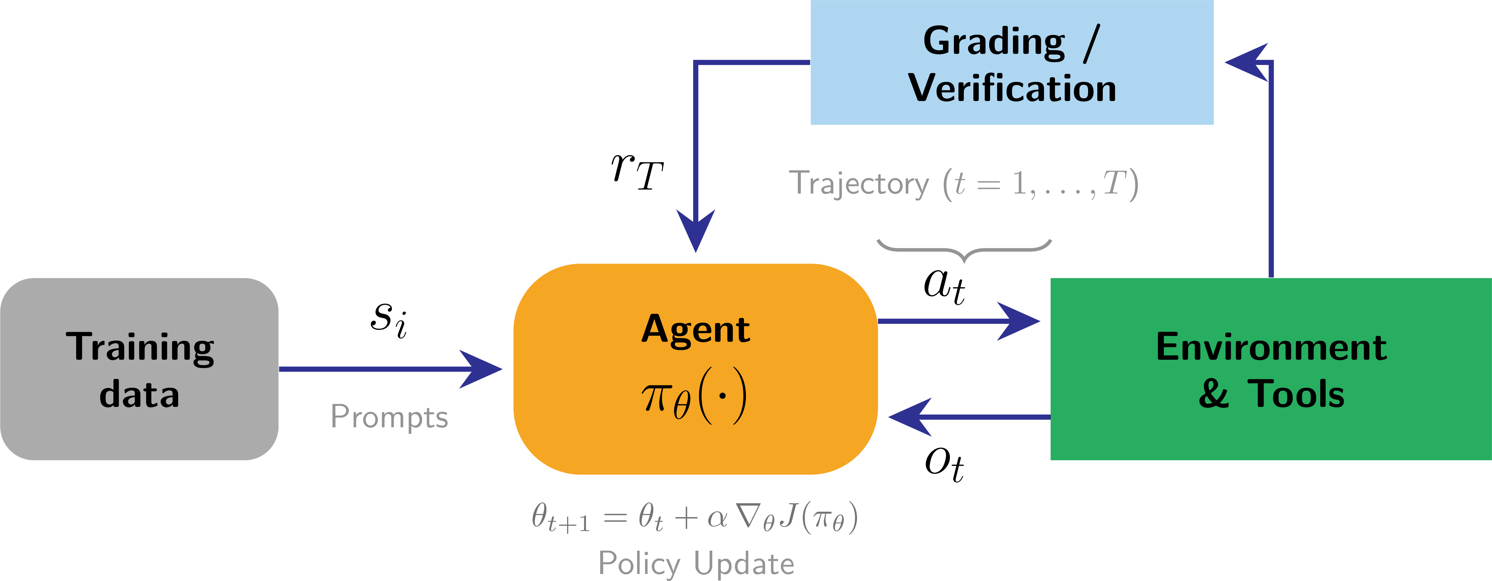
| MDP concept | RLVR | Agentic RL |
|---|---|---|
| State s_t | Prompt + tokens so far | Context (prompt + tokens + tool outputs), plus hidden environment state (files, services, other users) |
| Action a_t | Next token | Next token (many are tool calls) |
| Transition | Deterministic-ish: append token | More stochastic: the environment runs the call and appends its output |
| Episode | One prompt → completion | Many turns; Inkling 2 Small’s p99 rollout takes 4 hours |
| Terminal reward | Verifier on the final answer | Tests on the final state of the environment |
| Loss | Every completion token | Tool-output tokens are masked: the model must not learn to predict the environment |
Math RL needed prompts and answer checkers. Agentic RL needs environments: containers, real file systems, services, verification tests (Ivison et al., 2026). Building worlds for LLMs is hard.


The objective and its gradient:
The gradient says: for each sampled token, compute the direction in parameter space that makes it more likely (\nabla \log \pi), then scale by how much better than expected it was (\Psi_t).
The policy gradient derivation gives:
So we write a loss whose negative gradient is the policy gradient, treating each advantage A_i as a constant across the trajectory:
Gradient descent on L is gradient ascent on J.
In code, we compute the log-probs and let autodiff handle the gradient:
seq_log_probs = (token_log_probs * completion_mask).sum(dim=-1)
loss = -(seq_log_probs * advantages.detach()).mean()
loss.backward() # fills each parameter's .grad with ∇L
optimizer.step() # θ ← θ - η ∇L
loss.backward() runs backpropagation: it computes \partial L / \partial \theta for every parameter.
optimizer.step() applies the update.
The loss values themselves are often weird in RL (e.g. zero-centered distributions, rather than nice decreasing accuracy metrics of pretraining)
Most RL algorithms used today are variations on this computation.
The fundamental building block: per-token log-probabilities from the policy.
# Forward pass through the model
logits = model(input_ids).logits # (B, L, vocab_size)
# Autoregressive shift: logit at position t predicts token at t+1
logits = logits[:, :-1, :] # (B, L-1, vocab_size)
labels = input_ids[:, 1:] # (B, L-1)
completion_mask = completion_mask[:, 1:] # (B, L-1)
# Per-token log-probs
log_probs = logits.log_softmax(dim=-1)
token_log_probs = log_probs.gather(dim=-1, index=labels.unsqueeze(-1)).squeeze(-1) # (B, L-1)
# Per-sequence log-prob: sum over completion tokens
seq_log_probs = (token_log_probs * completion_mask).sum(dim=-1)
Everything in log-space to avoid numerical underflow from multiplying many small probabilities.
The simplest policy gradient loss:
# rewards: (B,) — one reward per sequence
# seq_log_probs: (B,) — sum of log-probs over completion tokens
# Baseline: average reward in the batch
baseline = rewards.mean()
advantages = rewards - baseline
# REINFORCE loss (negative because we minimize)
loss = -(advantages * seq_log_probs).mean()
TPositive advantage → increase probability. Negative → decrease.
(Aside: How we reduce per-token losses to a scalar — .mean() here — turns out to matter more than you’d expect. More in the book and lecture video.)
Policy-gradient theory is built on the assumption of on-policy data – from the current model weights in the training framework of the LLM.
As models get bigger, this is hard because: sampling is expensive, sampling is dominated by long-trail generations, most people use separate systems for inference v training, moving large model weights around is slow, inference weights can be further quantized for speed relative to training weights, multi-cluster deployments, etc.
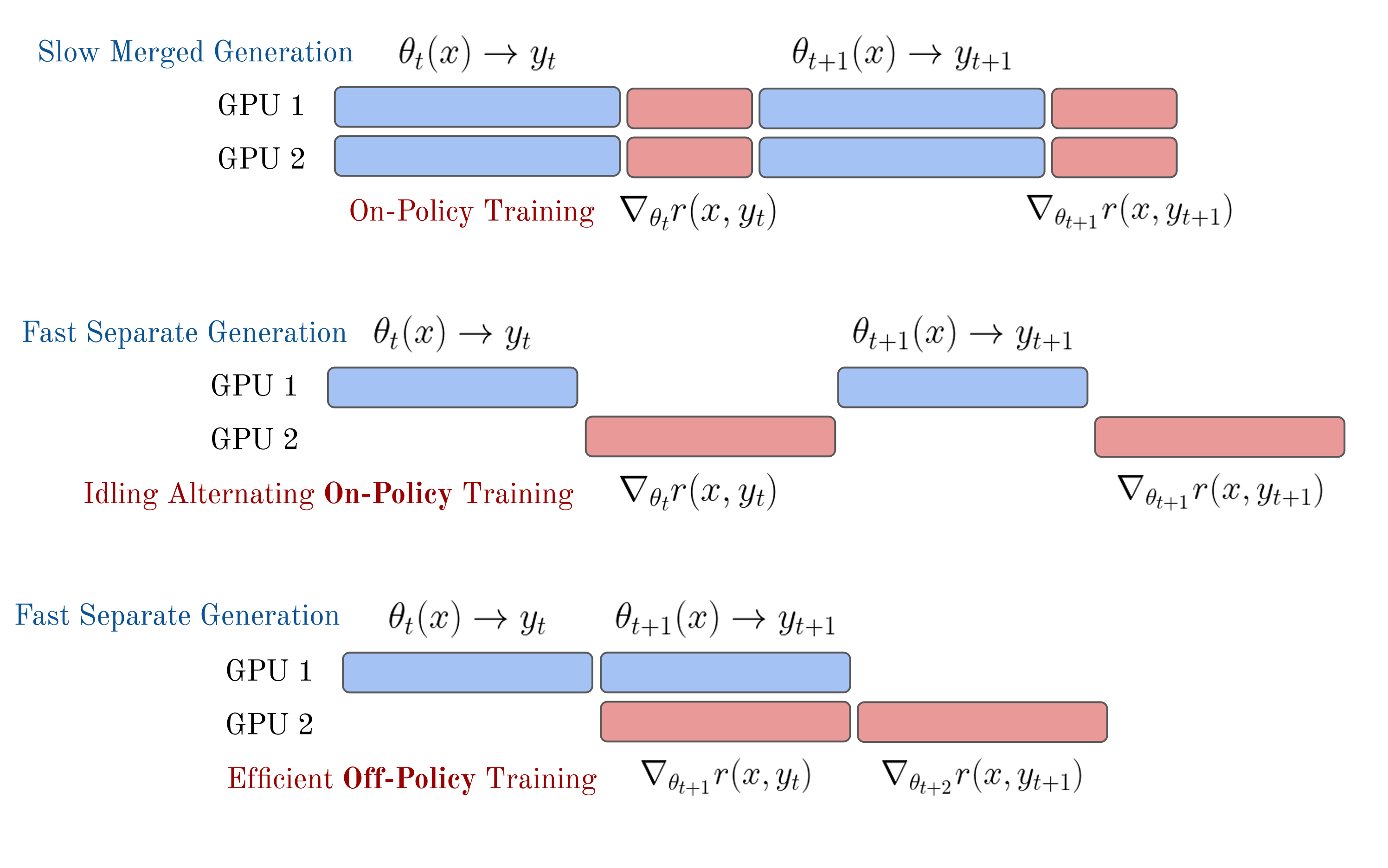
The default implementation for policy-gradient algorithms is on-policy execution: the generations from the language model are scored before updating the model.

Moving generation to an inference engine on its own GPUs makes it fast. To stay on-policy, each side waits for the other.

The common solution is to constantly run inference and training on separate GPU nodes. The model used for generation may be 1–N steps behind the training model.

This turns out to be mostly “fine” – but it can be taken too far.
Ideal / Theory (on-policy): generate → update → generate → update
Each batch of completions is scored and used for a short update window (one or a few epochs), then discarded.
Reality (async): generation and training overlap on different GPU groups for better throughput. The model used for generation may be 1–N steps behind the training model.
Tradeoff: perfect on-policy is slow (GPUs idle during generation or training). Slight staleness (how off-policy the data is) is usually fine.
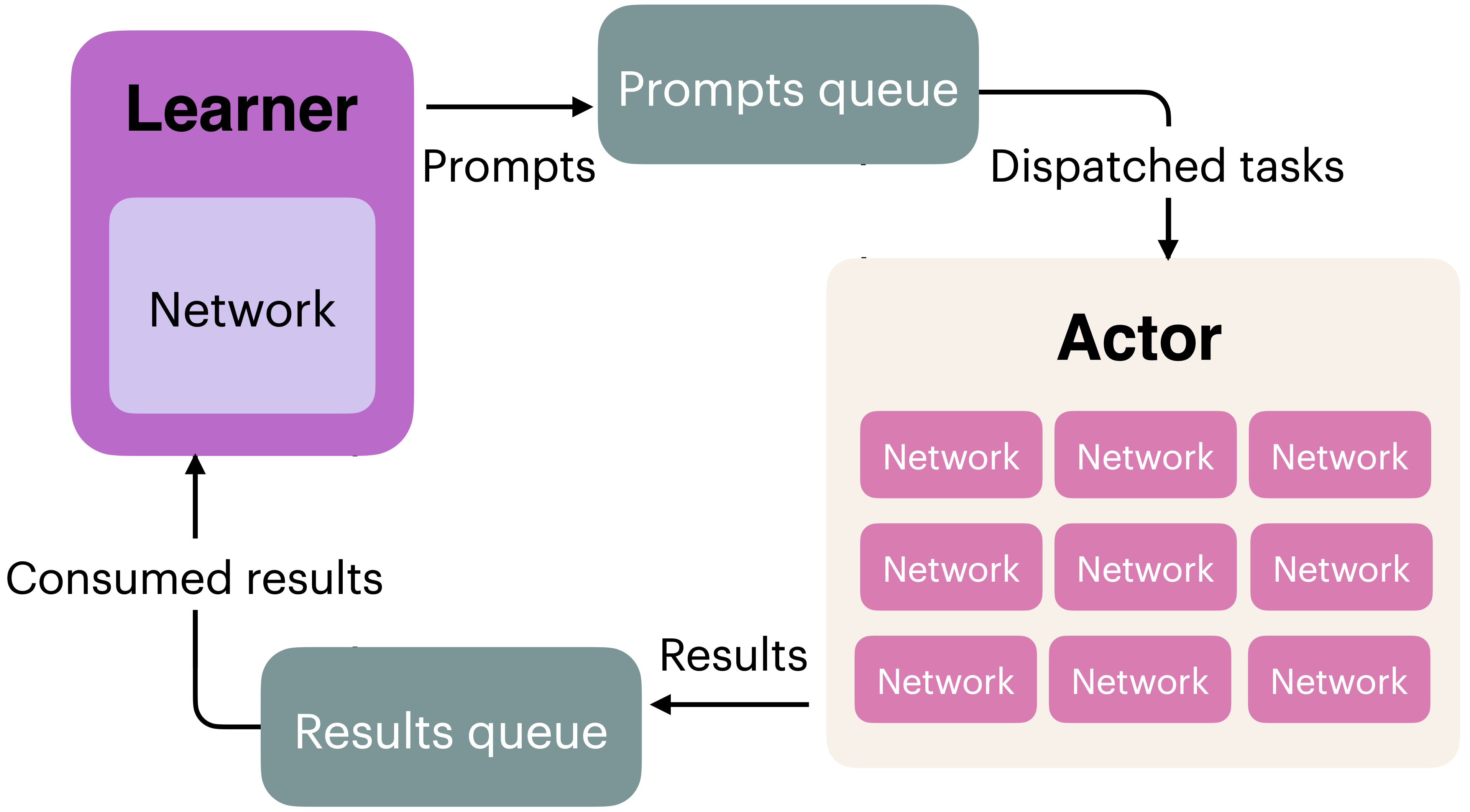
Modern RL for LLMs splits compute into two groups:
A process management library (e.g., Ray) coordinates data flow between them. Model weights are synced periodically from learner → actor.
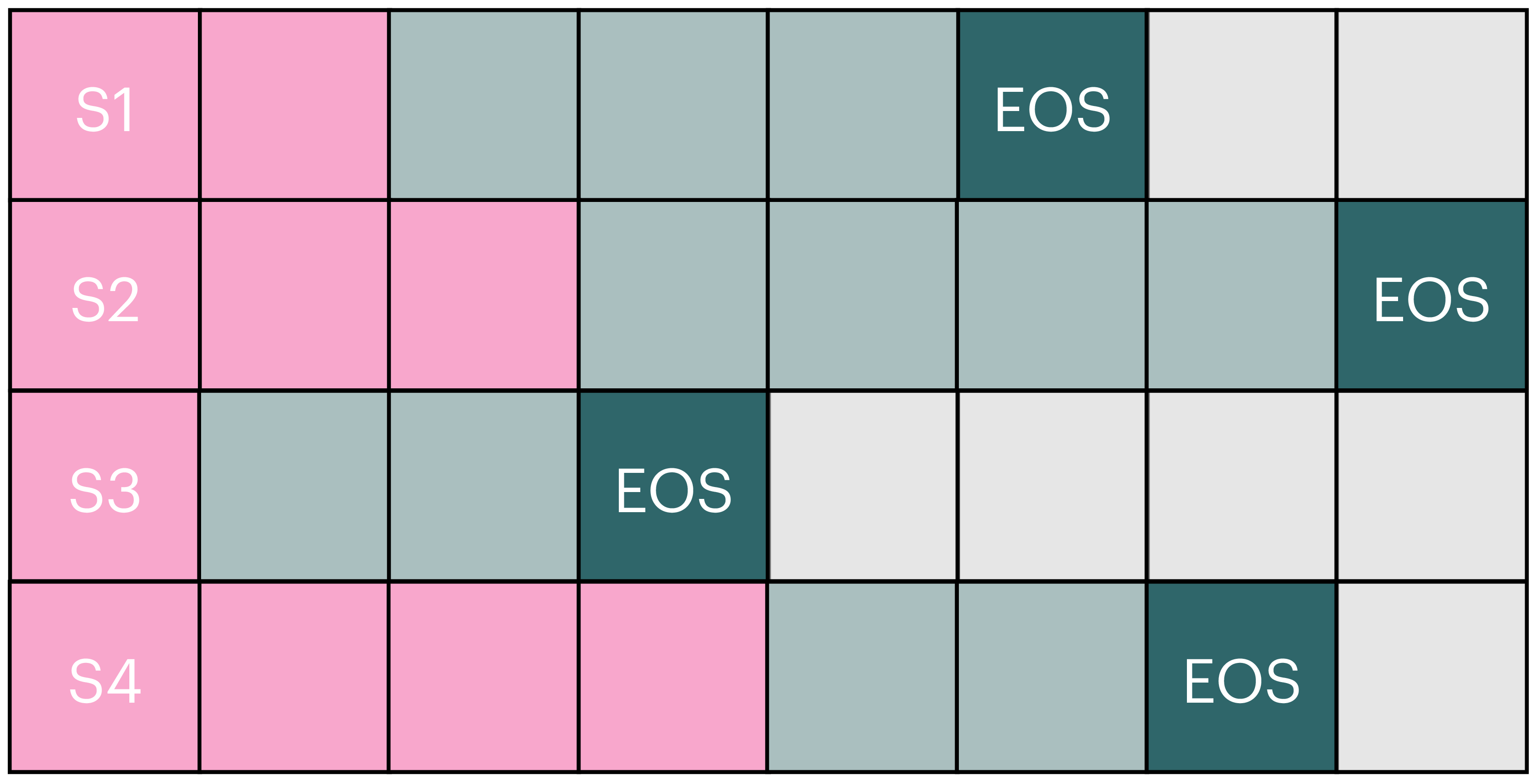
With static batching, each actor generates a whole batch and returns it only when the longest sequence finishes.

| Olmo 3 RL infrastructure | Tokens/s |
|---|---|
| Olmo 2 baseline | 881 |
| + continuous batching | 975 |
| + better threading | 1,358 |
| + inflight updates | 2,949 |
Continuous batching: start a new prompt as soon as a sequence finishes.
Inflight updates: load new weights without pausing generation or dropping the KV cache. The biggest speedup, but tokens in one completion now come from different weights.
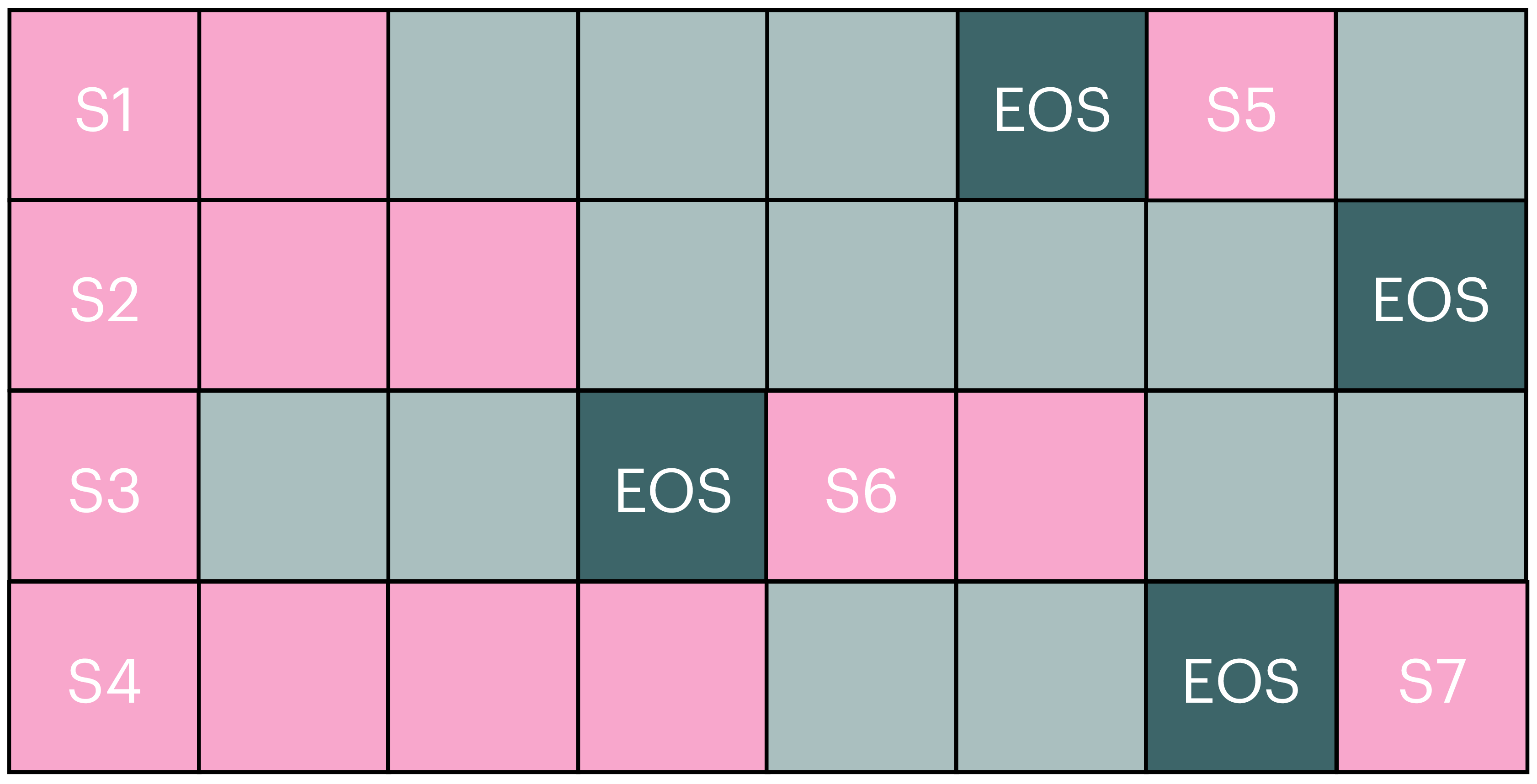
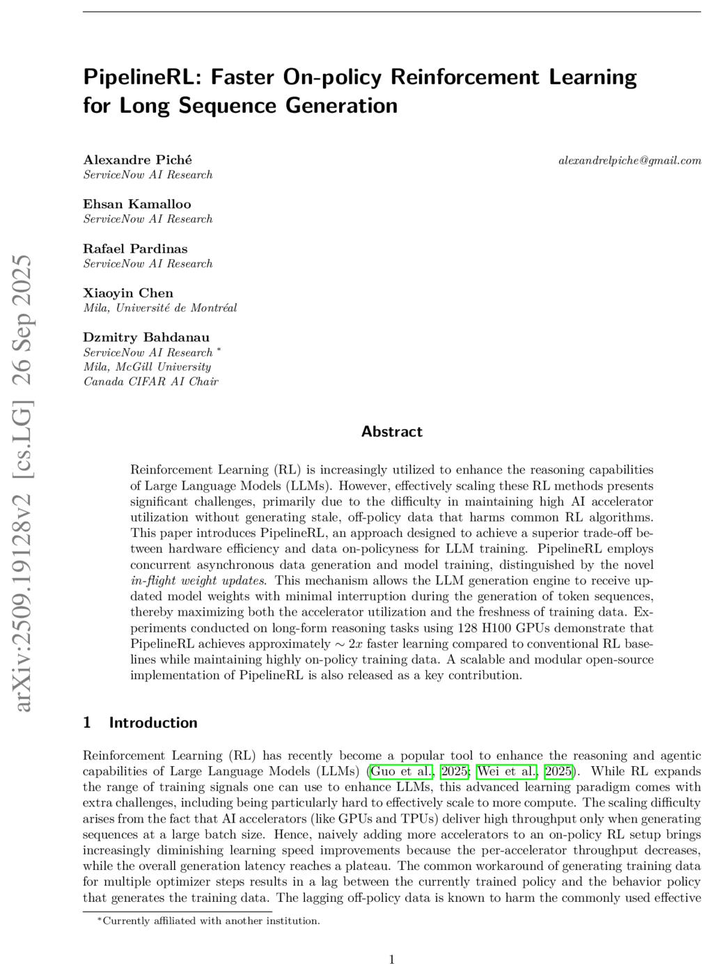
The canonical reference for inflight weight updates is PipelineRL (Piché et al., 2025).
# 1. Sample completions on the inference engine (pseudocode)
input_ids, completion_mask = sampler.generate(prompts, n=G)
# 2. Score them, then center within each group
rewards = verifier(prompts, input_ids) # (B*G,)
advantages = group_center(rewards, G) # (B*G,)
# 3. Recompute log-probs on the trainer, this time with gradients
logits = model(input_ids).logits[:, :-1, :]
token_logprobs = logits.log_softmax(-1).gather(
-1, input_ids[:, 1:].unsqueeze(-1)).squeeze(-1)
seq_logprobs = (token_logprobs * completion_mask[:, 1:]).sum(-1)
# 4. Update, then sync the new weights back to the sampler
(-(advantages * seq_logprobs).mean()).backward()
optimizer.step()
sampler.load_weights(model)
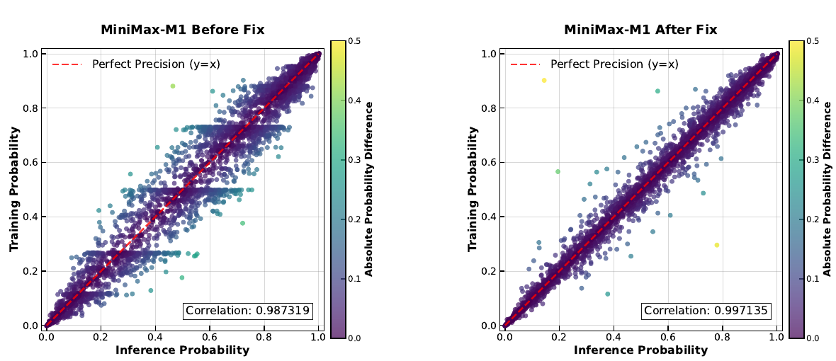
Steps 1 and 3 ask two different systems about the same tokens. Do they agree?
At one position, with prompt x and prefix a_{<t}, each system defines a next-token distribution:
Training-inference mismatch (TIM) is when q \neq p. There are two independent sources:

The gradient we want samples from the learner:
The gradient we compute samples from the sampler, but differentiates through the learner:
These differ whenever q \neq p, and the gap has two parts: the tokens are drawn from the wrong distribution, and so are the prefixes they follow.
Reweighting by the sequence ratio recovers the gradient exactly (Marek & Ryabinin, 2026):
But w can take very large values on rare tokens, which inflates the variance of the gradient.
Truncated importance sampling (Ionides, 2008) caps the per-token ratio at a constant C, trading a small bias for bounded variance in the policy gradient:
In practice, LLM RL systems apply TIS as a per-token correction weight on the policy-gradient loss:
# Shape: (B*G, L)
C = 2.0 # TIS cap
logratio = learner_logprobs - sampler_logprobs
logratio = logratio.clamp(-10.0, 10.0) # numerical safety
tis_weight = torch.exp(logratio).clamp(max=C) # one-sided truncation
# Use as a fixed correction weight on the per-token PG loss
per_token_pg_loss = per_token_pg_loss * tis_weight.detach()
TIS for the learner–sampler ratio has been adopted across major open-source RL frameworks (VeRL, TRL, OpenRLHF, SkyRL, OAT, and Open Instruct, which uses C = 2).
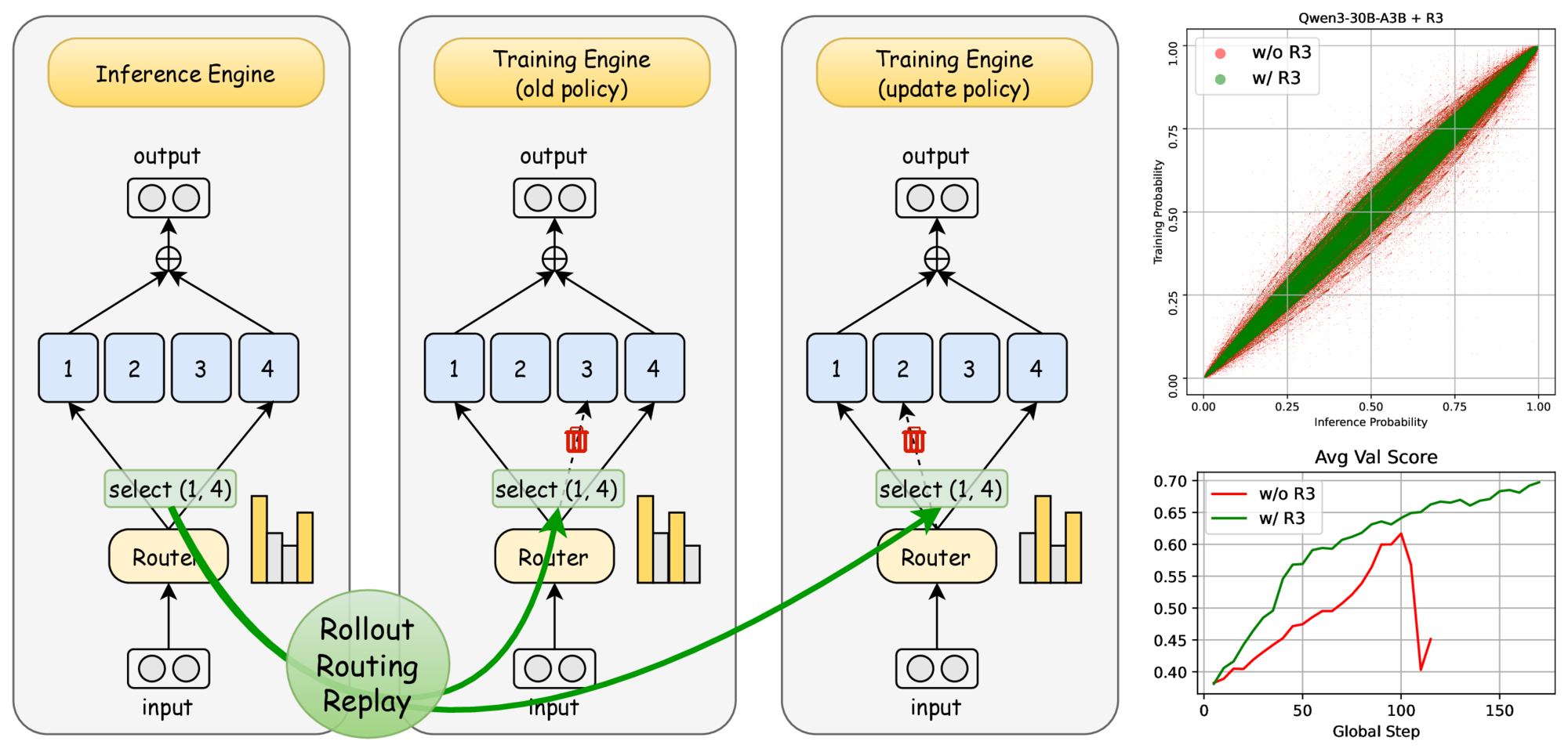
In mixture-of-experts (MoE) models, the trainer’s router can pick different experts than the sampler’s for the same token. Rollout Routing Replay (R3) records the experts chosen at inference and reuses them in the training forward passes.

The policy gradient for one completion:
Call each term the score of the token, \boldsymbol{\xi}_v = \nabla_\theta \log p_\theta(v \mid x, a_{<t}):
At one position, the expected score under the learner, written as a sum:
Shorthand: p_v = p_\theta(v \mid x, a_{\lt t}), the learner’s probability of token v at this position (\theta dropped for brevity); \mathcal{V} is the vocabulary.
Apply the log-derivative identity, p_v \nabla_\theta \log p_v = \nabla_\theta p_v:
Pull the gradient out of the sum. Probabilities sum to one:
This is why baselines are free: \mathbb{E}[b(x) \, \boldsymbol{\xi}_{a_t}] = b(x) \cdot \mathbf{0}. It relies on the expectation and the score using the same distribution.
Tokens now come from q, but the score is still computed through p. Define the expected score under the sampler:
Shorthand: q_v = q(v \mid x, a_{\lt t}) for the sampler and p_v = p_\theta(v \mid x, a_{\lt t}) for the learner (\theta dropped for brevity).
Apply the same log-derivative identity as before:
The weights are now q_v / p_v instead of 1, so the sum no longer collapses to \nabla_\theta 1 = \mathbf{0}. The expected score is zero when q = p, but not in general.
Start from the estimated gradient, and move the sum outside the expectation:
Sequences are sampled one token at a time, so split each term into the prefix, then the token and everything after it:
From here on, fix the prefix (context) and study the inner term. We write it as \mathbb{E}_q[A \, \boldsymbol{\xi}_{a_t}]. With the prefix fixed, the token a_t and the advantage A are both still random variables.
Use the covariance identity, \mathbb{E}[XY] = \mathbb{E}[X] \, \mathbb{E}[Y] + \text{Cov}(X, Y), starting on-policy, the expectation of the gradient:
Now the same identity under the sampler, where \mathbb{E}_q[\boldsymbol{\xi}_{a_t}] = \bar{\boldsymbol{\xi}}:
Only the covariance sees which tokens led to which outcomes. The drift depends on the advantages only through their mean – not per-token attribution.
The drift, \mathbb{E}_q[A] \, \bar{\boldsymbol{\xi}}, depends on the advantages only through their mean, so it moves the weights the same way regardless of which token was sampled.
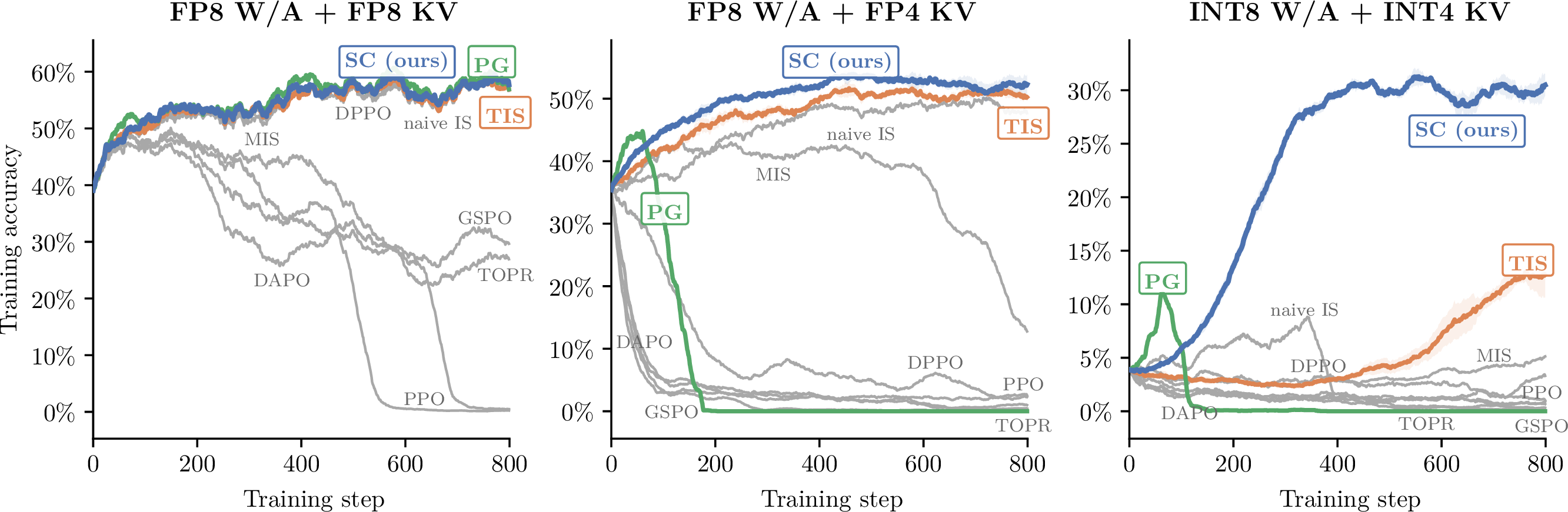
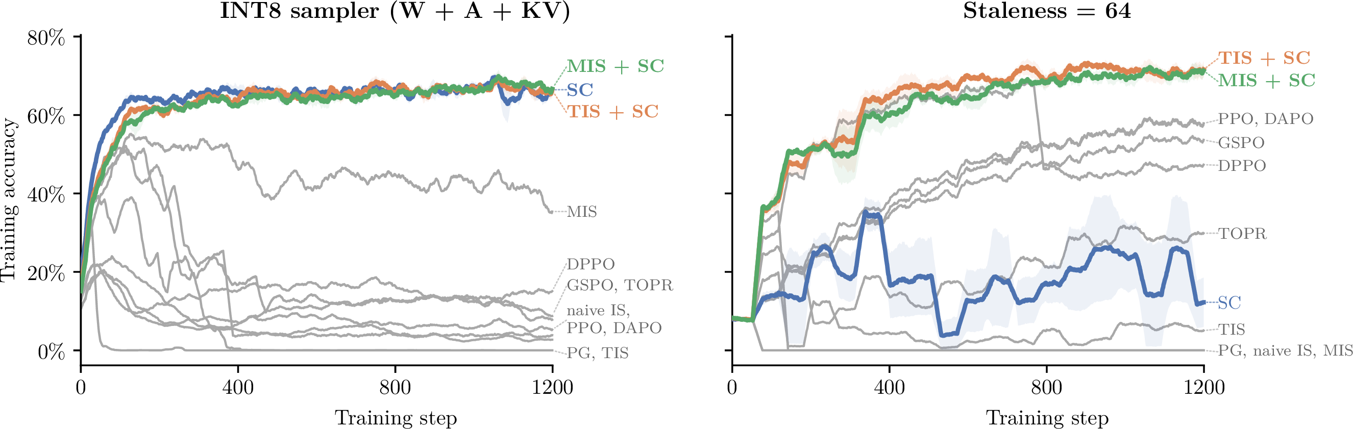
We don’t want that: in practice, it can pull the learner’s weights toward a stale and/or quantized sampler, causing potentially compounding instabilities.
Baselines center the reward. Score centering centers the per-token log-prob gradients (called “score” in statistics), subtracting its expected value under the sampler:
Recall: the score of token v is \boldsymbol{\xi}_v = \nabla_\theta \log p_\theta(v \mid x, a_{\lt t}), the gradient of its log-probability under the learner.
\bar{\boldsymbol{\xi}} is a sum over the whole vocabulary at a fixed prefix, so it is a constant with respect to the sampled token:
The centered score has zero mean under the sampler! which restores the property that made on-policy learning attractive. When q = p (on-policy), \bar{\boldsymbol{\xi}} = \mathbf{0} and the correction does nothing.
With the centered score, the policy-gradient estimate becomes:
Apply the covariance identity to the inner, per-token term:
The last step uses that a constant does not change a covariance: \text{Cov}(X, Y - c) = \text{Cov}(X, Y).


(Supposedly) Many labs are supposedly using StableReinforce, the loss Tinker added, rather than GRPO. This is unconfirmed, but the two are related.
The group advantages are nearly the same. GRPO normalizes each reward by the group mean and standard deviation:
REINFORCE with a group baseline is usually RLOO, which leaves each sample out of its own baseline:
Without the std, the two differ only by a constant scale. The bigger difference is the loss: GRPO usually wraps the advantage in PPO’s clipped ratio, while REINFORCE uses the plain log-prob loss.
Tinker’s docs describe the behavior, but not the main loss:
“In our internal post-training, this loss function has led to extremely stable training, even under highly off-policy async RL and low precision numerics.”
They do reveal a clue: sampling must record extra information, through record_stability_info=True.
Frontier losses are rarely published, so public ideas are rarely confirmed. Here, Martin Marek, the score centering paper’s first author, tried to recover the loss from its gradients alone.
Tinker does not expose the loss or the “stability info,” but it does let you take a step and download the weights.
Step 1: Recover the raw gradient. Tinker has no SGD, so use Adam with \epsilon = 10{,}000. This dominates Adam’s second moment:
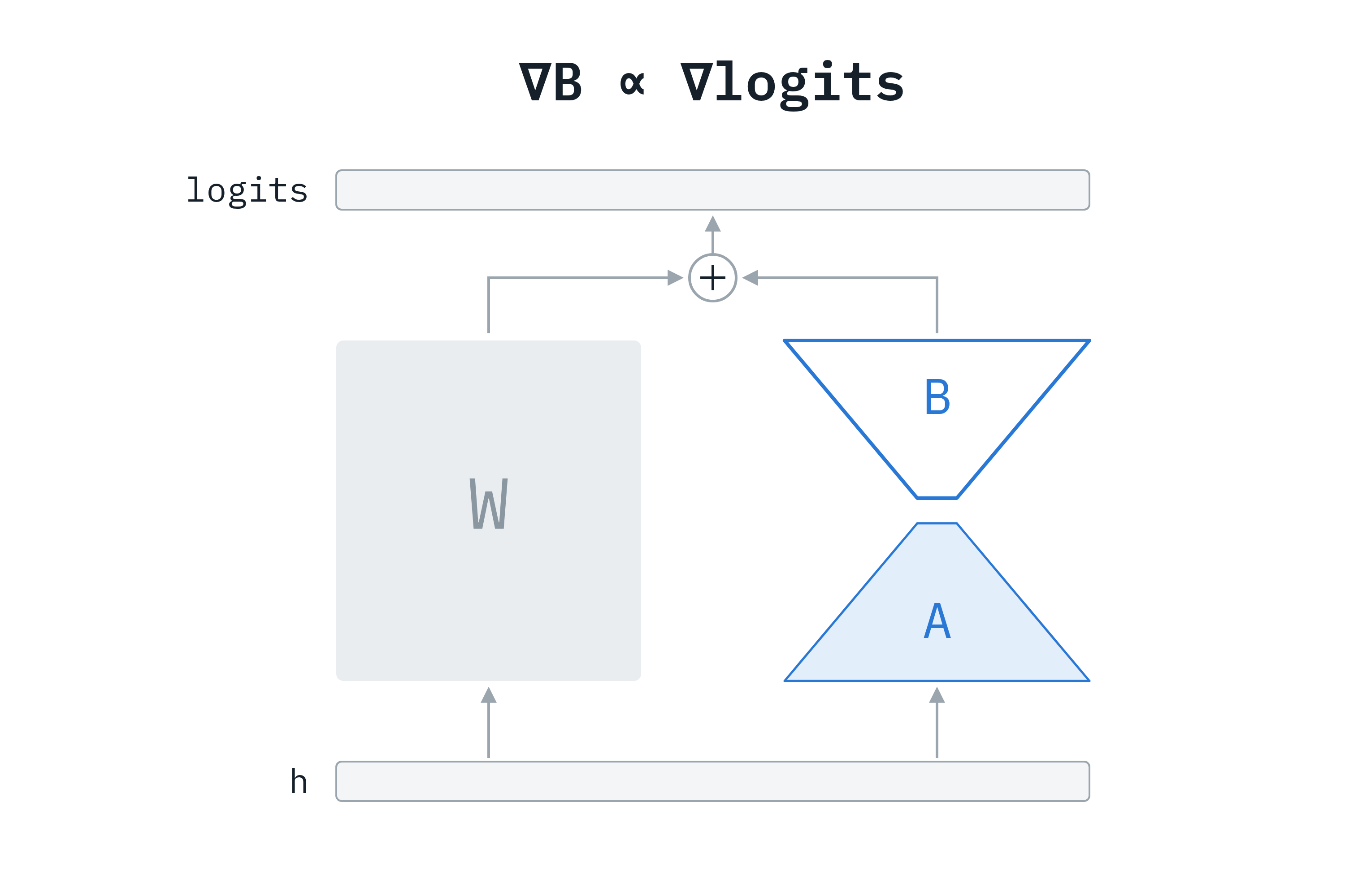
Step 2: Read it in logit space. Train a rank-1 LoRA adapter on the unembedding of Qwen3.5-4B. The gradient with respect to B equals the gradient with respect to the logits, up to scale.
For a single-token update:
The bars come in multiples of 1/8, and the third row, Reinforce with score centering, is identical.
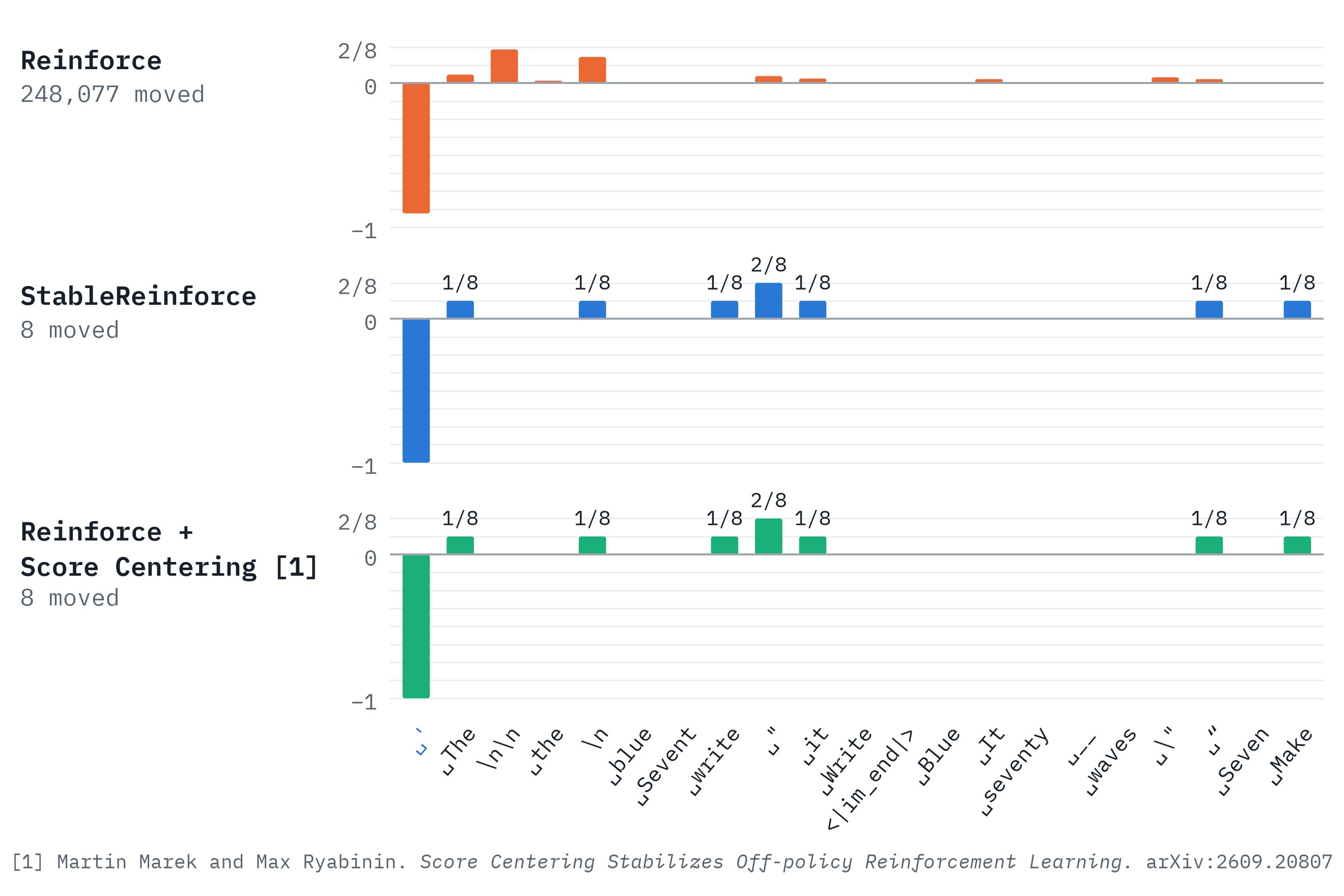
The plot shows gradients with respect to the logits z. For a softmax, the gradient of \log p_v is the one-hot vector e_v minus the probabilities:
Estimate \bar{\boldsymbol{\xi}} by drawing 8 tokens from the sampler, v_1, \dots, v_8 \sim q:
Subtract it from the score of the sampled token. The dense -p cancels exactly:
Flip the signs for a loss and this is the figure: -1 on the sampled token, +1/8 per draw.
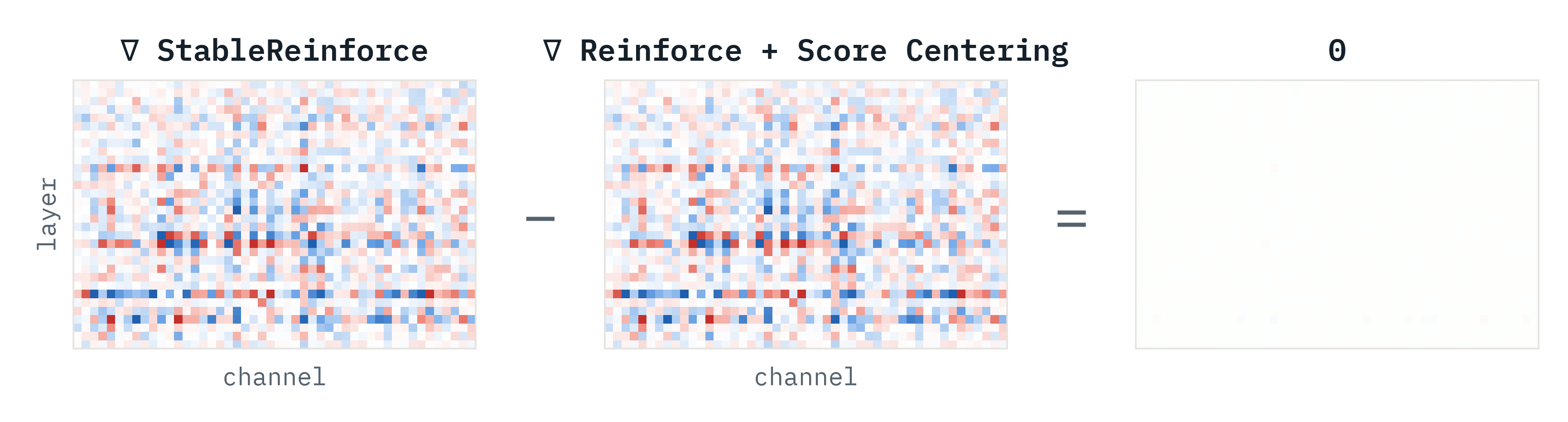
Hypothesis: StableReinforce is REINFORCE plus score centering, with the expected score computed over 8 randomly sampled tokens.
Test: Implement that as a custom Tinker loss, take an optimizer step, and compare. The gradients are within numeric precision across all layers.
Ripple-65B Preview, a 65B open-weight model from Ricursive (built on a lot of Olmo 3 infra!), names score centering in its post-training:
“Our mixed RL recipe uses truncated importance sampling, score centering, and linear length penalty with high-quality long-horizon synthetic environments.”
I have a lot of content expanding on this stuff!
![]()
The ratio between the two systems for a sampled token, and its log:
Tokens are sampled from q, so take the expectation under q:
Flip the sign to recognize the KL divergence:
If the systems agree, every \delta_t is zero. Otherwise, log-ratios are negative on average.
The ratio for a whole completion is the product of the token ratios:
Take the expectation under q, and apply the previous slide at each position:
This sum is the KL between the two sequence distributions, \text{KL}\big(q(a \mid x) \,\Vert\, p_\theta(a \mid x)\big), so it grows with length.
For illustration, a small per-token KL of 0.001 over 10{,}000 tokens gives a sequence KL of 10 nats. A typical weight is then near e^{-10} \approx 5 \times 10^{-5}.
In statistics, the score is the gradient of the log-likelihood with respect to the parameters. For one token v at one position:
Distilling toward a fixed teacher is harmless. It converges to the best fit of that teacher.
In online RL, the teacher moves with the student:
Not fully. Group centering makes advantages sum to zero over the rollouts of a prompt:
But drift arises at each prefix, and \mathbb{E}_q[A \mid x, a_{<t}] is generally not zero there:
Group centering shrinks drift relative to all-positive rewards, and it was the most stable reward setting in the paper’s online experiments. It does not eliminate drift.
We want a scalar whose gradient is A \, (\boldsymbol{\xi}_{a_t} - \bar{\boldsymbol{\xi}}).
The first piece is already a gradient, \boldsymbol{\xi}_{a_t} = \nabla_\theta \log p_{a_t}. For the second:
The sampler’s probabilities are logged values, so we mark them as constants with a stop-gradient and pull the gradient out:
Combine the two pieces, and multiply by -A:
The correction is one extra term in the REINFORCE loss from earlier:
# Learner: log-probs over the whole vocabulary, with gradients
learner_vocab_logprobs = logits.log_softmax(-1) # (B*G, L, V)
learner_logprobs = learner_vocab_logprobs.gather(
-1, tokens.unsqueeze(-1)).squeeze(-1) # (B*G, L)
# Sampler: logged at generation time, so it has no gradient path
sampler_probs = sampler_vocab_logprobs.exp() # (B*G, L, V)
# The gradient of `centering` is the expected score, s-bar
centering = (sampler_probs * learner_vocab_logprobs).sum(-1) # (B*G, L)
# advantages: (B*G, 1), broadcast to every token
per_token_loss = -advantages * (learner_logprobs - centering)
loss = ((per_token_loss * mask).sum(1) / mask.sum(1)).mean()
No ratios, no masks, and no clipping. On-policy, the gradient of centering is zero.
Computing \bar{\boldsymbol{\xi}} exactly needs the sampler’s next-token distribution at every position:
Instead, log only the sampler’s head H, its k most likely tokens at that position, with k = 128. Model the tail with the learner, rescaled to carry the sampler’s missing mass:
Substitute \hat{q} into the expected score, and split the sum into head and tail:
The zero-mean identity splits the same way, which rewrites the tail in terms of the head:
Substitute, and collect the terms. Only the k head tokens remain:
The paper reports that k = 128 and k = 32 both perform on par with the full vocabulary, at under 1% wall-clock overhead for k = 128.
# Logged during generation: sampler_topk_logprobs, sampler_topk_ids (B*G, L, k)
learner_logprobs = learner_vocab_logprobs.gather(-1, tokens[..., None])[..., 0]
head_logprobs = learner_vocab_logprobs.gather(-1, sampler_topk_ids) # (B*G, L, k)
learner_head_probs = head_logprobs.exp()
sampler_head_probs = sampler_topk_logprobs.exp()
# rho: the ratio of the sampler's tail mass to the learner's tail mass
sampler_tail = (1 - sampler_head_probs.sum(-1)).clamp_min(1e-6)
learner_tail = (1 - learner_head_probs.sum(-1)).clamp_min(1e-6)
rho = sampler_tail / learner_tail # (B*G, L)
# detach() is required: coef contains the learner's own probabilities
coef = (sampler_head_probs - rho[..., None] * learner_head_probs).detach()
centering = (coef * head_logprobs).sum(-1) # (B*G, L)
per_token_loss = -advantages * (learner_logprobs - centering)