Course Prereqs: The ML Foundations of LLM Post-Training

No prior reinforcement learning is assumed. We assume intro-ML comfort with losses, gradients, and probability, plus basic PyTorch tensor fluency. This deck is a refresher on autoregressive language models and the handful of ideas the course uses:

• Language models — autoregressive factorization of log-probs, the LM head, softmax, cross-entropy, and the tensor-shape anatomy
• Optimization — gradient descent, the training loop, pretraining → SFT
• Probability — KL divergence (with entropy), sigmoid and pairwise likelihood
• Reinforcement learning framing — the MDP setup and the goal of RL

The transformer backbone outputs a hidden state vector per token. The LM head is a final linear projection from the hidden dimension back to the vocabulary (tokenizer space).

• Hidden state \xrightarrow{\text{LM head}} logits (one score per vocab token)
• softmax over logits \rightarrow a probability distribution over the next token
• Sampling / argmax from that distribution \rightarrow the generated token

The same backbone can carry different heads for different jobs. In this course the first example is a reward-model head (Chapter 5) — same transformer, new head, new objective.

Softmax turns the logits z^{(t)} at step t into the next-token distribution — producing each per-token probability:

A whole sequence is the product of these terms (chain rule), and in log-space the product becomes a sum:

So every term in the sum is a log_softmax of the logits read off at the true token — which is exactly the (negative) cross-entropy loss at that position.

Why log-probs? Numerical stability (products of many small probabilities underflow), and sums are easier to differentiate than products.

Lectures discuss shifting logits, gathering target log-probs, and masking. Here is the whole path once, at the level of tensor shapes:

input_ids  ∈ ℕ^{B × L}          # INPUT TO MODEL -- token IDs, batch B, length L
   → model(input_ids).logits ∈ ℝ^{B × L × V}     # one vector per position, V = vocab
   → log_softmax + gather    ∈ ℝ^{B × (L-1)}     # log-prob of each observed token
   → (× completion_mask).sum ∈ ℝ^{B}             # one completion log-prob per sequence

Next: the same path in PyTorch, one line at a time.

logits = model(input_ids).logits            # (B, L, V): a score for every vocab token, at every position

logits = model(input_ids).logits            # (B, L, V): a score for every vocab token, at every position
logits = logits[:, :-1, :]                  # drop the last position — its prediction has no next token to score

logits = model(input_ids).logits            # (B, L, V): a score for every vocab token, at every position
logits = logits[:, :-1, :]                  # drop the last position — its prediction has no next token to score
labels = input_ids[:, 1:]                   # the target at each position is just the actual next token (the shift)

logits = model(input_ids).logits            # (B, L, V): a score for every vocab token, at every position
logits = logits[:, :-1, :]                  # drop the last position — its prediction has no next token to score
labels = input_ids[:, 1:]                   # the target at each position is just the actual next token (the shift)
completion_mask = completion_mask[:, 1:]    # shift the mask the same way so it lines up with labels (1 = completion)

logits = model(input_ids).logits            # (B, L, V): a score for every vocab token, at every position
logits = logits[:, :-1, :]                  # drop the last position — its prediction has no next token to score
labels = input_ids[:, 1:]                   # the target at each position is just the actual next token (the shift)
completion_mask = completion_mask[:, 1:]    # shift the mask the same way so it lines up with labels (1 = completion)
log_probs = logits.log_softmax(dim=-1)      # normalize logits into log-probabilities over the vocab -> (B, L-1, V)

logits = model(input_ids).logits            # (B, L, V): a score for every vocab token, at every position
logits = logits[:, :-1, :]                  # drop the last position — its prediction has no next token to score
labels = input_ids[:, 1:]                   # the target at each position is just the actual next token (the shift)
completion_mask = completion_mask[:, 1:]    # shift the mask the same way so it lines up with labels (1 = completion)
log_probs = logits.log_softmax(dim=-1)      # normalize logits into log-probabilities over the vocab -> (B, L-1, V)
token_log_probs = log_probs.gather(-1, labels.unsqueeze(-1)).squeeze(-1)  # read off the log-prob of each TRUE next token -> (B, L-1)

logits = model(input_ids).logits            # (B, L, V): a score for every vocab token, at every position
logits = logits[:, :-1, :]                  # drop the last position — its prediction has no next token to score
labels = input_ids[:, 1:]                   # the target at each position is just the actual next token (the shift)
completion_mask = completion_mask[:, 1:]    # shift the mask the same way so it lines up with labels (1 = completion)
log_probs = logits.log_softmax(dim=-1)      # normalize logits into log-probabilities over the vocab -> (B, L-1, V)
token_log_probs = log_probs.gather(-1, labels.unsqueeze(-1)).squeeze(-1)  # read off the log-prob of each TRUE next token -> (B, L-1)
seq_log_probs = (token_log_probs * completion_mask).sum(dim=-1)           # zero out prompt/pad, then sum per sequence -> (B,)

The one-token shift is the autoregressive step made literal: position t’s logits predict token t+1. Sum the per-token log-probs and loss.backward() — autodiff turns that sum into the corresponding sum of per-token gradients.

Masking is where silent bugs live in LLM code. Three different masks do three different jobs:

• Causal mask (built into decoder attention) — position t cannot attend to positions > t. This is what makes the model autoregressive; you never touch it in training code.
• Attention / padding mask — tells attention to ignore padding tokens (variable-length sequences batched together). Shape (B, L).
• Completion / loss mask — 1 only on completion tokens; the loss is multiplied by it before summing. Prompt tokens condition the prediction but contribute no loss.

Get the completion mask wrong and you either train on the prompt (wastes gradient on tokens you can’t change) or on padding (trains on noise).

Generation samples/searches over \pi_\theta — same weights, many ways to pick each token:

• Greedy — take \arg\max_v P_\theta(v \mid x_{<t}) each step. Deterministic but myopic: a locally best token can doom the sequence.
• Beam search — keep the top-b partial sequences by cumulative log-prob, expand and prune to b. Great for low-entropy tasks (translation), bland for open-ended text.
• Temperature sampling — y_t \sim \mathrm{softmax}(z_t / T). Higher T → more diverse, lower T → sharper toward greedy.
• Truncated sampling — sample only from the top-k tokens, or the smallest set with cumulative mass \ge p (top-p / nucleus).
• Lookahead search (MCTS & friends) — score simulated future continuations (often with a value/reward model) before committing — decode-time cousin of inference-time reasoning.

Key split: the distribution \pi_\theta vs the procedure that samples it.

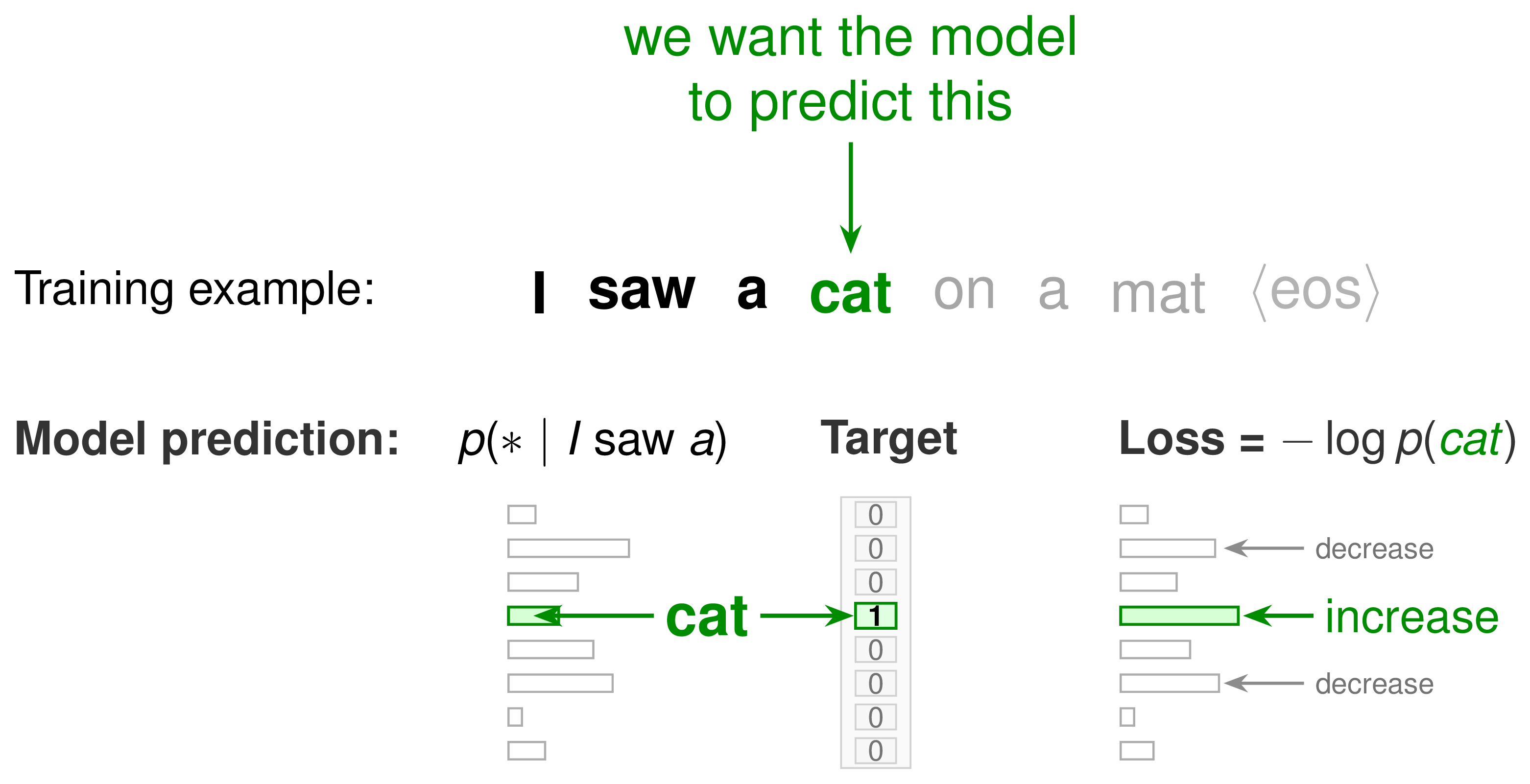
At each position, cross-entropy compares the model’s predicted distribution to the true next-token label q_t. That label is a one-hot at the actual token x_t, so the sum over the vocabulary collapses to a single term:

So the “comparison to the true token” is just the one-hot picking out one log-prob. Summing over positions and averaging over data gives the LM loss — equivalently, the negative log-likelihood (NLL):

“Predict the next token” is supervised learning — the label is just the next token in the sequence.

Training repeats one step:

• \theta — model parameters, \eta — learning rate, \nabla_\theta \mathcal{L} — gradient of the loss
• AdamW and related adaptive optimizers are standard for LM training (adaptive, momentum-based) rather than plain SGD
• Training is measured in optimizer steps / tokens; epochs are a useful unit for finite fine-tuning datasets. The learning-rate schedule matters as much as the rate itself

The basic backprop loop is shared across pretraining, mid-training, and fine-tuning — what differs is masking, sampling, batching, data construction, and systems, not the optimizer.

The boundary at the end of pretraining is fuzzy and very important to post-training:

• Pretraining — next-token cross-entropy on massive raw web/code data; every token contributes to the loss.
• Mid-training — the annealing / high-quality-data phase at the very end of pretraining, before any instruction data. Quality ramps up here. Could be considered part of post-training, but often isn’t discussed.
• SFT (supervised fine-tuning) — still cross-entropy, but now on instruction–response pairs with a completion mask: only the response tokens contribute to the loss, the prompt merely conditions. The model learns to respond, not just continue text.

Modern post-training pipelines start from a mid-trained checkpoint, so this is where the course’s story effectively begins.

The Kullback–Leibler divergence measures how one distribution differs from another:

Three things to remember:

• Asymmetric — \mathcal{D}_{\text{KL}}(p\|q) \neq \mathcal{D}_{\text{KL}}(q\|p); direction matters
• Non-negative, and 0 only when p = q
• The central object of alignment: the RLHF KL penalty (Lectures 3–4) keeps the policy close to its SFT start, and the DPO loss (Lecture 6) is derived from a KL-regularized reward-maximization objective

Related: Entropy H(p) = -\sum_i p_i \log p_i is the uncertainty of a distribution (uniform = high, peaked = low). It shows up in definitions, derivations, and understanding of these systems. Very similar computation.

You will see KL in essentially every alignment lecture.

Three quantities, one information-theoretic picture (measured in nats with \ln, bits with \log_2):

• Entropy H(p) = -\sum_i p_i \log p_i — the average surprise of samples from p; the irreducible cost to encode them. Uniform = high, peaked = low.
• Cross-entropy H(p, q) = -\sum_i p_i \log q_i — the cost of encoding samples from p using a code built for the wrong distribution q.
• KL divergence \mathcal{D}_{\text{KL}}(p \,\|\, q) = \sum_i p_i \log \frac{p_i}{q_i} — precisely that extra cost of using q instead of p.

They are one identity:

So minimizing cross-entropy is minimizing KL to the truth — H(p) is fixed by the data. In LM training the label p is one-hot, so H(p)=0 and cross-entropy = KL = NLL. In RLHF the KL term is instead added on purpose, to keep the policy near its reference.

Over sequences the sum behind KL is intractable — but KL is an expectation, so estimate it by Monte Carlo: average the log-ratio over samples drawn from the policy.

• The integrand is just the log-probability ratio on each rollout you already generate.
• The naive average (\hat k_1 = \log\frac{\pi_\theta}{\pi_{\text{ref}}}) is unbiased but high-variance and can go negative on a finite sample.
• RLHF uses the low-variance, always-\ge 0 k_3 estimator \hat k_3 = r - 1 - \log r, with r = \tfrac{\pi_{\text{ref}}}{\pi_\theta} (Schulman, 2020).

This is the practical face of the information theory: approximate a target distribution from samples, paying for the estimate in variance rather than an intractable sum.

A preference (“response y_w is better than y_l”) is a binary outcome, so a score difference is squeezed through a sigmoid into a probability:

Three things to recognize:

• sigmoid converts a score difference into a binary probability
• only relative reward differences matter — shifting both rewards by a constant changes nothing
• -\log \sigma(\cdot) is just binary negative log-likelihood

Lecture 2 derives this Bradley–Terry model in full to train a reward model; Lecture 6 reuses the exact same \sigma(\Delta r) shape inside DPO.

Reinforcement learning studies an agent acting in a Markov decision process (\mathcal{S}, \mathcal{A}, P, r, \gamma):

The policy is the LM, factorized over tokens:

The goal of RL is to choose policy parameters \theta that maximize expected reward under the policy itself:

A human preference (or a verifier) is a single scalar at the end of a response:

• Sparse — one label per whole response, not per token
• Delayed — the quality of a token depends on the whole completion
• No token-level target — and ordinary gradients can’t pass back through the discrete sampled token

So there is no cross-entropy target for “preferred.” Policy gradients optimize the expected evaluator score anyway — first by learning that signal as a reward model, then by optimizing it. That is the whole motivation for RLHF.

Everything in this deck is the basic machinery — probabilities, losses, gradients, and sampling. Post-training is what you get when you point that machinery at a pretrained model with richer feedback than raw next-token prediction:

• Demonstrations (“produce this response”) → supervised fine-tuning
• Preferences (“make this response more likely than that one”) → reward modeling or preference optimization (DPO)
• Rewards (“sample responses that score highly”) → reinforcement learning (PPO, GRPO, RLVR)
• Constraints (“don’t drift too far from where you started”) → regularization, especially the KL penalty

Different data and different objectives; the same underlying goal:

Change the model’s distribution over responses toward behavior we want.

That is what the rest of this course is about.

• RL — Sutton & Barto, Reinforcement Learning: An Introduction; David Silver’s UCL course; UC Berkeley CS285
• Language models from scratch — Sebastian Raschka, Build a Large Language Model (From Scratch)
• The book’s own reference — Appendix A (Definitions) covers the language-modeling overview, KL, and RL vocabulary used throughout

Go down rabbit holes, skip around, and chase what excites you — the course is built for that.