Lecture 10: Regularization in RL, Why RL Generalizes, and Why SFT Forgets

rlhfbook.com

Nathan Lambert

Post-training course. Chapter 15.

How do these optimizers change the distributions of the models? How do we control it?

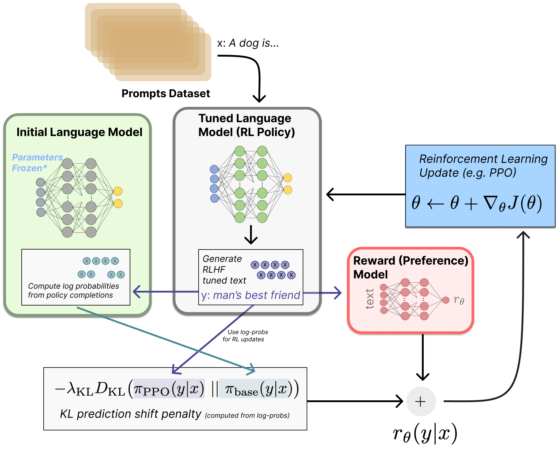
Recall: The RLHF process

The RL step maximizes reward from the reward model minus a penalty for drifting from the reference model.

This lecture is about that penalty – and what happens with and without it.

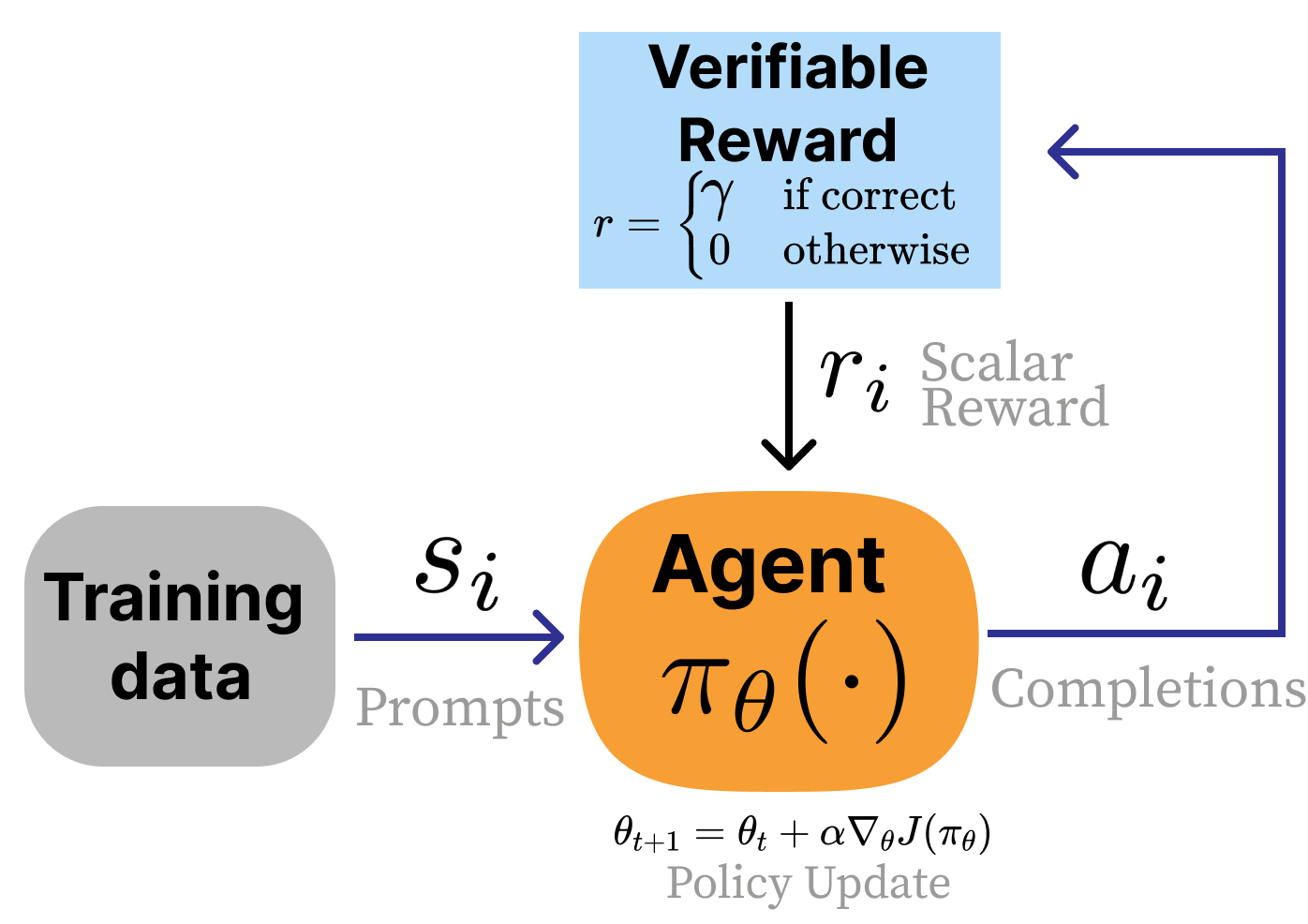
The RLHF training pipeline -- the RL step optimizes the policy against the reward model, held close to the reference model by a KL penalty. — The RLHF training pipeline – the RL step optimizes the policy against the reward model, held close to the reference model by a KL penalty.

RLVR has regularization too, but different best practices

Same RL loop, different reward source: a verification function instead of a reward model.

Reasoning models (before tool use) often dropped the KL penalty to enhance learning.

With the emergence of large-scale tool-use, regularization is coming back into vogue – but aimed at drift from the sampling distribution, not a KL penalty to a reference model (more on this at the end of the lecture).

RLVR uses a verification function instead of a reward model, but the RL loop -- and the regularization question -- is the same. — RLVR uses a verification function instead of a reward model, but the RL loop – and the regularization question – is the same.

This lecture

How we control optimization pressures on models explicitly.

How the math of the optimizers we use changes the shapes of the models.

The plan

The KL penalty that controls RL
The two directions of KL divergences
Why RL generalizes better than SFT
Other related work

Aside: Watch lecture 9 first

Lecture 9 slidesrlhfbook.com

Slides – yes, these are the real slides, in a slide.

Lecture 9 videowww.youtube.com

Watch on YouTube

Part 1: The explicit KL penalty

A KL penalty to the reference model controls reward

The canonical LLM reward function:

r = r_\theta - \lambda_{\text{KL}} \, D_{\mathrm{KL}}\!\left( \pi_{\text{RL}}(y \mid x) \,\|\, \pi_{\text{ref}}(y \mid x) \right)

KL control for RL predates LLMs: dialogue agents (Jaques et al., 2017), then fine-tuning pretrained models (Jaques et al., 2020).
This penalty is a reverse KL – estimated by sampling from the policy and scoring against the reference. It punishes the policy for putting mass where the reference would not.
“KL distance” is the optimization distance spent (colloquially – KL is not a true metric).
In practice, the above \lambda is often written as \beta.

Measuring KL in practice

Sampling from P turns the definition into an expectation:

D_{\mathrm{KL}}(P \,\|\, Q) = \mathbb{E}_{x \sim P}\left[ \log P(x) - \log Q(x) \right]

Practitioners watch the KL curve during training – a very large KL usually means a bug or a broken model.
Lower-variance estimators (k_1, k_2, k_3) came up in Q&A 2 (Schulman, 2020).

# sample from the policy
tokens = model.generate(inputs)

# score sampled tokens under both models
logprobs     = log_softmax(model.forward(tokens).logits)
ref_logprobs = log_softmax(ref_model.forward(tokens).logits)

# log-probs of the tokens actually generated
token_lp     = gather(logprobs, tokens)
ref_token_lp = gather(ref_logprobs, tokens)

# sequence-level difference approximates KL
kl_approx = token_lp.sum(-1) - ref_token_lp.sum(-1)

What the curves look like in a real run

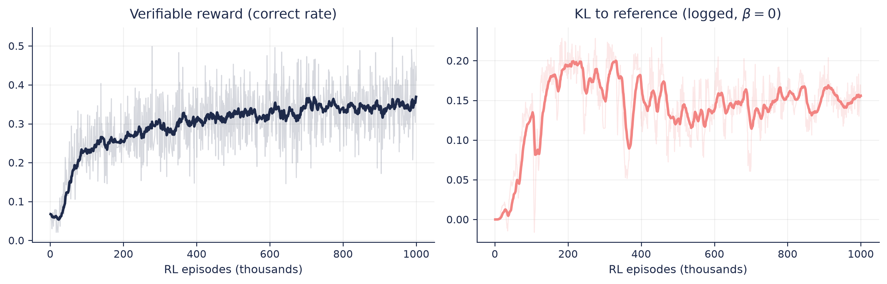
An OLMo-2-7B GRPO run, RL directly on the base model (R1-Zero-style, no SFT), from open-instruct (public W&B logs): over ~1M episodes the verifiable reward climbs while the logged KL to the reference rises and then wanders. This run has β = 0. This is a healthy shape.

Static or dynamic KL penalties? β began as a feedback controller

The first RLHF-on-LMs paper did not fix β. It picked a target KL and let a controller chase it:

e_t = \operatorname{clip}\!\left( \frac{\mathrm{KL}(\pi_t, \pi_{\text{ref}}) - \mathrm{KL}_{\text{target}}}{\mathrm{KL}_{\text{target}}},\, -0.2,\, 0.2 \right), \qquad \beta_{t+1} = \beta_t \left(1 + K_\beta\, e_t\right)

A “log-space proportional controller” (their words), with K_\beta = 0.1: KL too high → β grows and pulls the policy back; too low → β shrinks and frees it up. Runs with different seeds land on the same KL budget, making experiments comparable.
The idea is older than RLHF: PPO’s original adaptive KL penalty variant doubled or halved β around a target (Schulman et al., 2017), and constrained RL later made the controls framing explicit with full PID controllers on the penalty multiplier (Stooke et al., 2020).
Modern practice swung back to a small static β – or, in many RLVR reasoning recipes, no KL term at all.

Ziegler et al., 2019

Static or dynamic KL penalties? β began as a feedback controller

The first RLHF-on-LMs paper did not fix β. It picked a target KL and let a controller chase it:

e_t = \operatorname{clip}\!\left( \frac{\mathrm{KL}(\pi_t, \pi_{\text{ref}}) - \mathrm{KL}_{\text{target}}}{\mathrm{KL}_{\text{target}}},\, -0.2,\, 0.2 \right), \qquad \beta_{t+1} = \beta_t \left(1 + K_\beta\, e_t\right)

Read the code: the original controller (lm-human-preferences, 2019) · TRL’s AdaptiveKLController (v0.11.4 – deleted in the modern rewrite) · open-instruct today: a static beta = 0.05, applied directly in the loss.

Ziegler et al., 2019

Part 2: RL optimization is a reverse KL minimization

The reward penalty and the optimization shape are two different things

We started with a penalty on the RL setup: a term added to the reward, with a coefficient you tune (or control).

This next part is about the shape of RL optimization and how it relates to KL as well. It comes down to “which direction of KL” – that is set by where the samples come from:

SFT samples from data (or a separate teacher model) → minimizing its loss is exactly minimizing a forward KL.
RL samples from itself → with the penalty on, maximizing the objective is exactly a reverse-KL minimization toward a reward-tilted reference. This is only true with the KL penalty in the optimization (does not apply to all RLVR results)… but on-policy sampling still biases RL toward KL-minimal solutions. More on that later.

RL is reverse KL

Start from the KL-regularized objective (the one our RL trainers optimize):

\max_\pi\; \mathcal{J}_{\text{RL}}(\theta) = \mathbb{E}_{x \sim \mathcal{D},\, y \sim \pi(\cdot \mid x)}\left[ r(x, y) \right] - \beta\, D_{\mathrm{KL}}\!\left(\pi(\cdot \mid x) \,\|\, \pi_{\text{ref}}(\cdot \mid x)\right)

Dividing by -\beta and normalizing turns the objective into a single KL – minimized exactly when \pi equals the optimal policy \pi_\star. Lecture 6 walked this same path (the starting point of DPO):

\pi_\star(y \mid x) = \frac{1}{Z(x)}\, \pi_{\text{ref}}(y \mid x)\, \exp\!\left(\tfrac{1}{\beta}\, r(x,y)\right)

Read \pi_\star as the reward-tilted reference (AI suggested name, I couldn’t come up with something better): take \pi_{\text{ref}} and multiply each completion’s probability by \exp(r/\beta), then renormalize (that is all Z(x) does). The “tilt” shifts probability mass toward high-reward completions while staying inside the reference’s support – large \beta tilts barely at all, small \beta concentrates on the highest-reward completions.

Chen et al., 2025

RL is reverse KL

Now expand the reverse KL to \pi_\star, substituting \log \pi_\star = \log \pi_{\text{ref}} - \log Z(x) + \tfrac{1}{\beta} r(x,y):

D_{\mathrm{KL}}(\pi_\theta \,\|\, \pi_\star) = \mathbb{E}_{x \sim \mathcal{D},\, y \sim \pi_\theta}\left[ \log \pi_\theta(y \mid x) - \log \pi_\star(y \mid x) \right] \qquad \text{definition; samples from } \pi_\theta

\phantom{D_{\mathrm{KL}}(\pi_\theta \,\|\, \pi_\star)} = \mathbb{E}_{x \sim \mathcal{D},\, y \sim \pi_\theta}\left[ \log \pi_\theta - \log \pi_{\text{ref}} + \log Z(x) - \tfrac{1}{\beta}\, r(x,y) \right] \qquad \text{substitute } \log \pi_\star

\phantom{D_{\mathrm{KL}}(\pi_\theta \,\|\, \pi_\star)} = -\tfrac{1}{\beta}\,\mathbb{E}\left[r(x,y)\right] + D_{\mathrm{KL}}\!\left(\pi_\theta \,\|\, \pi_{\text{ref}}\right) + \underbrace{\log Z(x)}_{\text{constant}} \qquad \text{regroup the terms}

\phantom{D_{\mathrm{KL}}(\pi_\theta \,\|\, \pi_\star)} \propto -\tfrac{1}{\beta}\, \mathcal{J}_{\text{RL}}(\theta) \qquad \text{drop the constant}

\boxed{\ \max_\theta\, \mathcal{J}_{\text{RL}}(\theta) \iff \min_\theta\, D_{\mathrm{KL}}(\pi_\theta \,\|\, \pi_\star)\ }

With the penalty included, RL doesn’t just use a reverse KL – the whole objective is one, pointed at the reward-tilted reference policy.

Chen et al., 2025

SFT is forward KL

Now the comparison point. SFT trains on a fixed dataset – the samples come from the data distribution, call it \pi_{\mathcal{D}}, which makes it the other KL direction:

\begin{aligned} D_{\mathrm{KL}}(\pi_{\mathcal{D}} \,\|\, \pi_\theta) &= \mathbb{E}_{(x,y) \sim \mathcal{D}} \left[ \log \pi_{\mathcal{D}}(y \mid x) - \log \pi_\theta(y \mid x) \right] && \text{definition; samples are the data} \end{aligned}

\begin{aligned} &= \underbrace{\mathbb{E}_{(x,y) \sim \mathcal{D}}\left[ \log \pi_{\mathcal{D}}(y \mid x) \right]}_{-H(\pi_{\mathcal{D}}),\ \text{constant in } \theta} \; - \; \mathbb{E}_{(x,y) \sim \mathcal{D}}\left[ \log \pi_\theta(y \mid x) \right] && \text{split the expectation} \end{aligned}

\begin{aligned} &= -H(\pi_{\mathcal{D}}) + \mathcal{L}_{\text{SFT}}(\theta) \;\propto\; \boxed{\ \mathcal{L}_{\text{SFT}}(\theta)\ } && \text{the NLL term is the SFT loss} \end{aligned}

Same gradients, same minimum: minimizing the SFT loss is minimizing forward KL to the data distribution.

SFT and RL are the two directions of KL

This is very reminiscent of Lecture 7 (on-policy distillation), with both directions of KL at play. Post-training math repeats itself:

Forward KL – supervised fine-tuning (aka standard KL):

D_{\mathrm{KL}}(\pi_{\mathcal{D}} \,\|\, \pi_\theta) = \mathbb{E}_{y \sim \pi_{\mathcal{D}}}\!\left[\log \tfrac{\pi_{\mathcal{D}}(y)}{\pi_\theta(y)}\right]

Samples come from the target (a fixed dataset).

Mass-covering: wherever the target has mass and \pi_\theta \to 0, the loss blows up – the model must spread to cover everything.

Reverse KL – reinforcement learning:

D_{\mathrm{KL}}(\pi_\theta \,\|\, \pi_\star) = \mathbb{E}_{y \sim \pi_\theta}\!\left[\log \tfrac{\pi_\theta(y)}{\pi_\star(y)}\right]

Samples come from the policy itself.

Mode-seeking: only penalized where it places mass, so it concentrates on high-reward modes.

Recall, Lecture 7: The same two directions in distillation

The distillation version, verbatim from Lecture 7 – teacher \pi_T in place of the target. Sampling completions from the student is what puts \pi_\theta on the left of the KL:

Offline KD / SFT (forward KL) – the expectation is over the teacher, z \sim \pi_T (off-policy: a fixed teacher dataset):

D_{\mathrm{KL}}(\pi_T \,\|\, \pi_\theta) = \mathbb{E}_{z \sim \pi_T}\!\left[\log\frac{\pi_T(z)}{\pi_\theta(z)}\right]

Mass-covering – weighted by teacher mass: wherever the teacher has mass and \pi_\theta \to 0, the log-ratio blows up, so the student must cover everything the teacher might say.

On-policy distillation (reverse KL) – the expectation is over the student, z \sim \pi_\theta (on-policy: you sample the model you’re training):

D_{\mathrm{KL}}(\pi_\theta \,\|\, \pi_T) = \mathbb{E}_{z \sim \pi_\theta}\!\left[\log\frac{\pi_\theta(z)}{\pi_T(z)}\right]

Mode-seeking – weighted by the student’s own mass: penalized only where it puts probability the teacher dislikes, so it collapses onto the teacher’s modes. Lecture 7 deferred why reverse KL is better to this lecture.

Part 3: Why RL generalizes more

“SFT memorizes, RL generalizes”

Controlled study: post-train on one task, evaluate under a rule shift (i.e., small modifications of the problem to test out-of-distribution) (Chu et al., 2025).

GeneralPoints: reach 24 by combining four cards with +,-,\times,\div; test with shift to the face-card rule (train: J/Q/K = 10; test: 11/12/13).
V-IRL: visual navigation; test with shift from absolute (north/east) to relative (left/right) directions.

On V-IRL, RL improves out-of-distribution accuracy 80.8% → 91.8%. SFT collapses it 80.8% → 1.3% – destroying spatial reasoning the base model already had.

RL-based post-training carries implicit regularization from its on-policy structure alone. SFT is more brittle.

Paper: arxiv.org/abs/2501.17161

Chu et al., 2025

Which direction should forget less?

The naive read: forward KL is mass-covering, so SFT should preserve every mode – while mode-seeking RL should collapse onto one and forget the rest.

Is this correct?

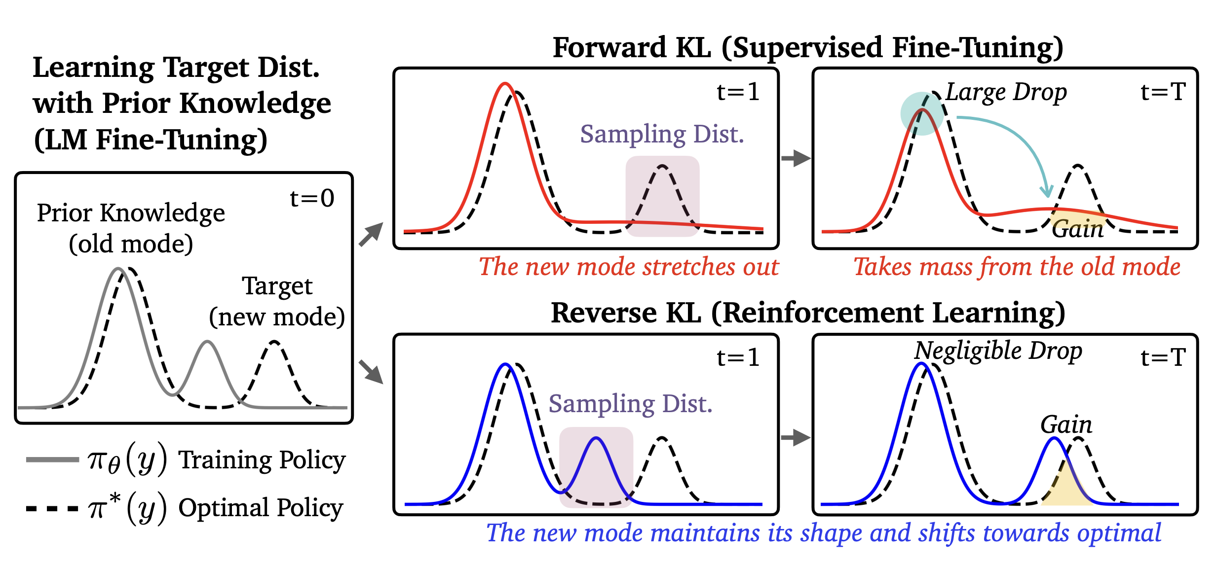
Which direction should forget less?

That intuition assumes a unimodal policy – LLMs are multimodal. Paper: arxiv.org/abs/2510.18874

Chen et al., 2025

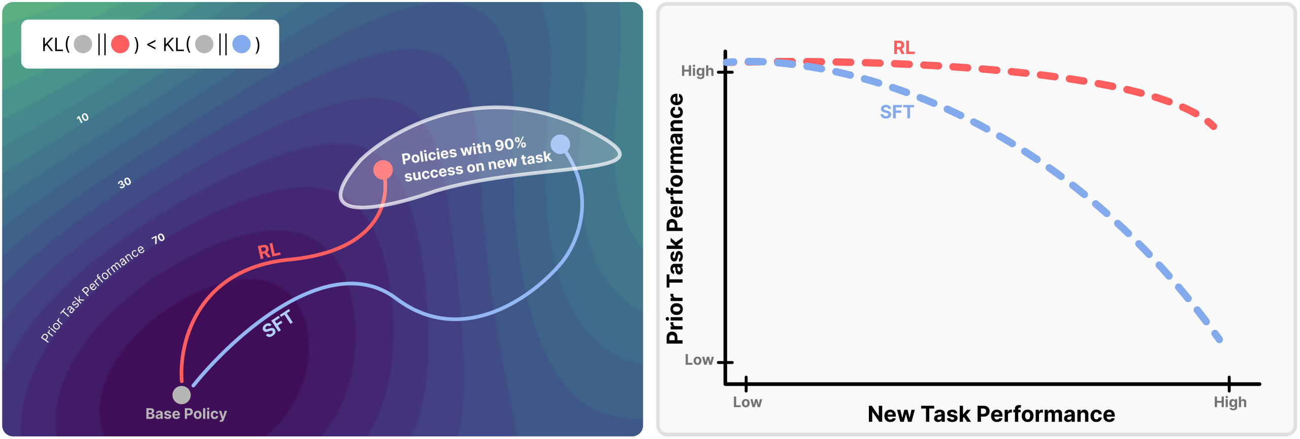
RL’s razor: Lower KL drift for equivalent performance

“Among the many high-reward solutions for a new task, on-policy methods such as RL are inherently biased toward solutions that remain closer to the original policy in KL divergence.”

Forgetting tracks KL drift: \text{Forgetting} \approx f\!\left(\mathbb{E}_{x \sim \tau}\!\left[D_{\mathrm{KL}}\!\left(\pi_0 \,\|\, \pi\right)\right]\right) with R^2 = 0.96 – measured on the new task’s data. A cheap forgetting predictor.
The ablation: on-policy data fully accounts for the difference – negative gradients have no discernible effect. Paper: arxiv.org/abs/2509.04259

Among policies that solve the new task, RL converges to those closest in KL to the base model -- yielding higher prior-task retention at matched new-task performance. Shenfeld et al., 2026 (CC-BY). — Among policies that solve the new task, RL converges to those closest in KL to the base model – yielding higher prior-task retention at matched new-task performance. Shenfeld et al., 2026 (CC-BY).

Shenfeld et al., 2026

Part 4: Other tools to control optimization

Other regularization in the wild

Most of these are scaffolding: added to stabilize one setup, simplified away in the next model generation.

Pretraining next-token pred. gradients (InstructGPT): add \gamma\, \mathbb{E}_{x \sim \mathcal{D}_{\text{pretrain}}}\left[\log \pi_{\text{RL}}(x)\right] to the objective, “to fix the performance regressions on public NLP datasets” (Ouyang et al., 2022).
NLL alongside DPO: \mathcal{L}_{\text{DPO+NLL}} = \mathcal{L}_{\text{DPO}} + \alpha\, \mathcal{L}_{\text{NLL}} keeps the chosen text high-likelihood in absolute terms, not just relatively better (Pang et al., 2024).
Margin loss for reward models (Llama 2): -\log \sigma\!\left(r_{\theta}(y_c) - r_{\theta}(y_r) - m(y_c, y_r)\right), where the margin m comes from annotator rating deltas – the Likert scales from Lecture 8 (Touvron et al., 2023).

2026: The trust region / KL pen. is moving on

Tool use is changing what regularization has to do. In agentic recipes, the KL-to-reference penalty is disappearing:

GLM-5 removes it outright – “to accelerate RL improvement” (GLM-5 Team et al., 2026). Kimi does not use one either: the K2 → K3 recipes ship with no KL penalty and no reference policy at all (Moonshot AI, 2026).
In our TMax terminal-agent recipe we measured the trade-off: a small KL reduced the severity of collapse but lowered reward, so the final recipe is \beta = 0 (Ivison et al., 2026).
TMax paper summarizes the change in numerical issues we are battling: 20+ turn trajectories, async/partial rollouts, and train-vs-inference engine mismatch make drift from the sampler the binding failure, not drift from init. (In TMax, instabilities increase past 10 assistant turns and were absent below 5 (Ivison et al., 2026).)

A trust region on the sampling distribution

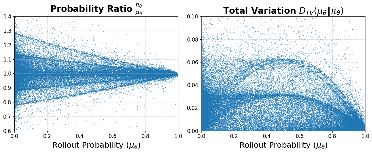
DPPO (Divergence Proximal Policy Optimization) masks tokens by a directly estimated divergence between the rollout and training policies (binary Total Variation), instead of PPO’s per-token ratio clip (Qi et al., 2026).

The per-token ratio is a noisy one-sample estimate of that divergence. GLM’s IcePop (GLM-5 Team et al., 2026) and Kimi’s log-ratio interval (Moonshot AI, 2026) do the same job: gradients masked, not clipped.

This is where the eye of regularization is today – algorithmic updates rather than KL penalties.

The motivation, from the DPPO paper: for the same rollout tokens, per-token probability ratios (left) explode at low probabilities while the directly-estimated TV divergence (right) stays stable. Qi et al., 2026.

Qi et al., 2026

Takeaways

The KL penalty is the explicit control: a reverse KL, estimated on the policy’s own samples.
The KL-regularized RL objective is a reverse KL minimization – mode-seeking toward a reward-tilted reference policy – while SFT is the forward direction, mass-covering toward the data.
Even with no penalty, on-policy RL is implicitly regularized – SFT memorizes, RL generalizes.

Verifiable rewards are much less prone to overoptimization than reward models! Hence, regularization is changing and the KL penalty is playing a smaller role.

The course so far

Prerequisites review
Overview (ch. 1-3)
IFT, reward models & rejection sampling (ch. 4, 5, 9)
RL: Motivation & math (ch. 6)
RL: Implementation & practice (ch. 6)
The rise of reasoning models (ch. 7)
Direct preference optimization (ch. 8)

Synthetic data & modern post-training (ch. 12)
Preferences & preference data (ch. 10-11)
Over-optimization & RLHF’s bad reputation (ch. 14, app. B)
Regularization (ch. 15) – today
Evaluation (ch. 16) – next (tentative)
Basics of tool-use (ch. 13) – hopefully?

Thank you

Questions / discussion are encouraged!

If you have a second to subscribe and/or share my content with a friend, it helps massively on getting the word out.

Contact: [email protected]

Newsletter: interconnects.ai

rlhfbook.com

Built withnatolambert/colloquium252 stars

References (1/2)

Chen, H., Razin, N., Narasimhan, K., and Chen, D.. “Retaining by Doing: The Role of On-Policy Data in Mitigating Forgetting.” 2025. [link]

Chu, T., Zhai, Y., Yang, J., Tong, S., Xie, S., et al.. “Sft memorizes, rl generalizes: A comparative study of foundation model post-training.” International Conference on Machine Learning (ICML), 2025.

GLM-5 Team, Zeng, A., Lv, X., Hou, Z., Du, Z., et al.. “GLM-5: From Vibe Coding to Agentic Engineering.” 2026. [link]

Ivison, H., Yin, J., Shao, R., Xiao, T., Lambert, N., et al.. “TMax: A Simple Recipe for Terminal Agents.” arXiv preprint arXiv:2606.23321, 2026. [link]

Jaques, N., Gu, S., Bahdanau, D., Hern\''andez-Lobato, J., Turner, R., et al.. “Sequence tutor: Conservative fine-tuning of sequence generation models with kl-control.” International Conference on Machine Learning, 2017.

Jaques, N., Shen, J., Ghandeharioun, A., Ferguson, C., Lapedriza, A., et al.. “Human-centric dialog training via offline reinforcement learning.” Conference on Empirical Methods in Natural Language Processing (EMNLP), 2020.

Moonshot AI. “Kimi K3: Open Frontier Intelligence.” 2026.

Ouyang, L., Wu, J., Jiang, X., Almeida, D., Wainwright, C., et al.. “Training language models to follow instructions with human feedback.” Advances in Neural Information Processing Systems, 2022.

References (2/2)

Pang, R., Yuan, W., Cho, K., He, H., Sukhbaatar, S., et al.. “Iterative reasoning preference optimization.” Advances in Neural Information Processing Systems (NeurIPS), 2024.

Qi, P., Zhou, X., Liu, Z., Pang, T., Du, C., et al.. “Rethinking the Trust Region in LLM Reinforcement Learning.” 2026. [link]

Schulman, J., Wolski, F., Dhariwal, P., Radford, A., and Klimov, O.. “Proximal Policy Optimization Algorithms.” arXiv preprint arXiv:1707.06347, 2017.

Schulman, J.. “Approximating KL Divergence.” 2020.

Shenfeld, I., Pari, J., and Agrawal, P.. “RL's Razor: Why Online Reinforcement Learning Forgets Less.” The Fourteenth International Conference on Learning Representations, 2026. [link]

Stooke, A., Achiam, J., and Abbeel, P.. “Responsive safety in reinforcement learning by PID Lagrangian methods.” International Conference on Machine Learning, 2020.

Touvron, H., Martin, L., Stone, K., Albert, P., Almahairi, A., et al.. “Llama 2: Open foundation and fine-tuned chat models.” arXiv preprint arXiv:2307.09288, 2023.

Ziegler, D., Stiennon, N., Wu, J., Brown, T., Radford, A., et al.. “Fine-tuning language models from human preferences.” arXiv preprint arXiv:1909.08593, 2019.