Lecture 3: Reinforcement Learning Motivation & Math
Nathan Lambert
Post-training course. Chapter 6, Part 1
Lecture 3: Reinforcement learning (mostly the math)
- Introduction
- Key related works
- Training overview
- Instruction tuning
- Reward models
- Reinforcement learning
- Reasoning
- Direct alignment
- Rejection sampling
- What are preferences
- Preference data
- Synthetic data & CAI
- Tool use
- Over-optimization
- Regularization
- Evaluation
- Product & character
- A. Definitions
- B. Style & information
- C. Practical issues
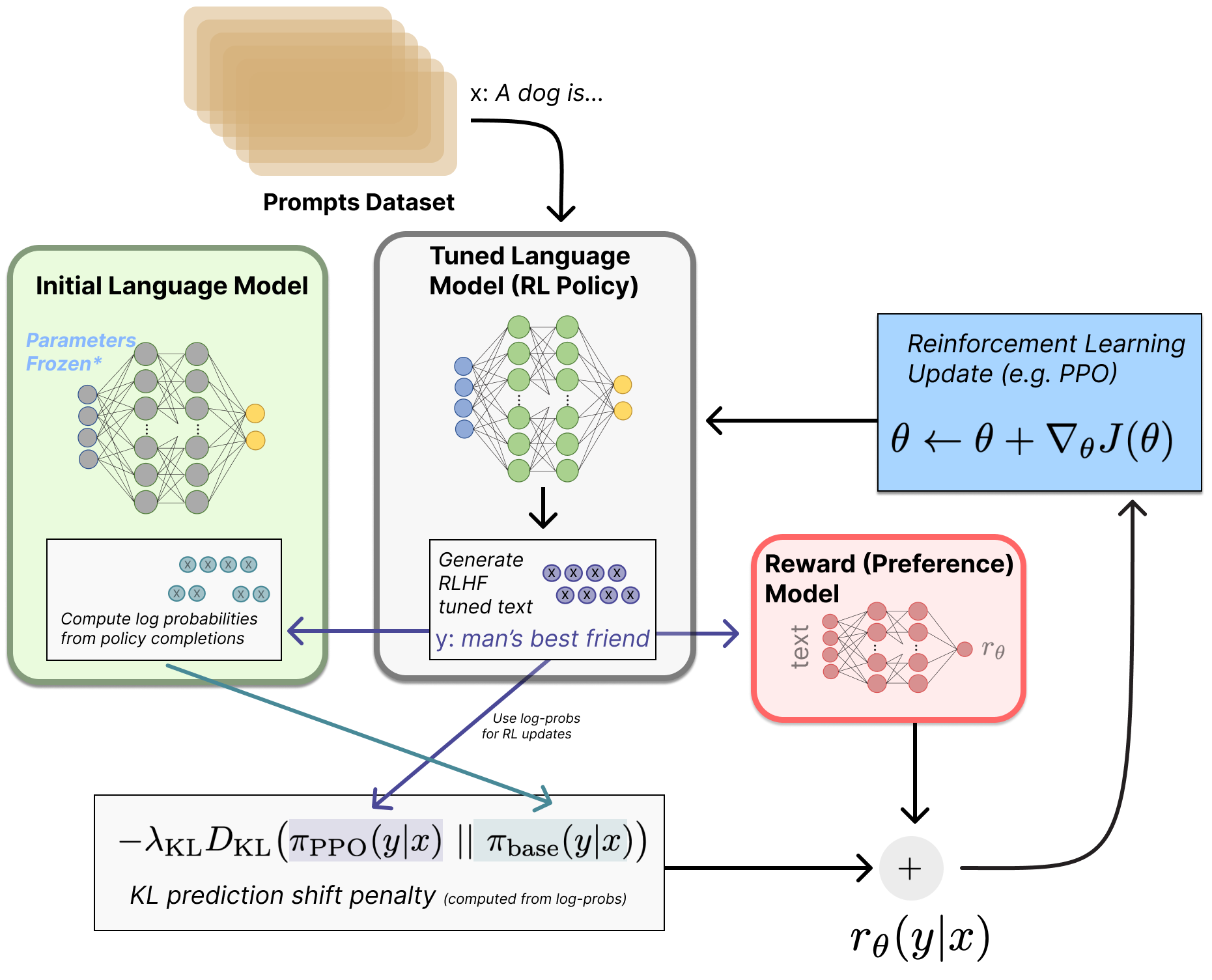
Where we are in the pipeline
After instruction tuning and training a reward model, the RL step updates the policy against a learned reward signal.
System diagram view.

Where we are in the pipeline
After instruction tuning and training a reward model, the RL step updates the policy against a learned reward signal.
RLHF optimization view.
What this lecture covers
This lecture covers the math and theory of RL for language models. The next lecture covers implementation.
- Motivation — why RL training matters
- RL foundations review — MDP, return, value functions, policy gradient objective
- Policy gradient derivation — log-derivative trick, step by step
- REINFORCE & RLOO — the simplest policy gradient algorithms
- PPO — trust regions, clipping, GAE, value functions
- GRPO & modern variants — GSPO, CISPO, and the trend toward simplicity
- Comparison — strengths, weaknesses, questions
An under-documented benefit of RL
In lecture 2, we covered rejection sampling and later we’ll cover direct alignment algorithms (like DPO). They’re simpler, but RL has hard to measure benefits.
Implementing RL is far more complex infrastructure, but the gradient updates it provides “generally help the model a lot.” This is hard to quantify, but:
- RL can “fix” rough edges on a model — making outputs more robust, better formatted, and more compatible with serving frameworks like vLLM
- RL operates on a narrow prompt distribution and tends not to “squash” general capabilities — it can be applied surgically to improve specific behaviors without degrading others
Overall, RL losses on language models are robust, scalable, effective, and flexible, which opened large new fields of experimentation. The original method that started us down this path was RLHF work.
Why RL matters
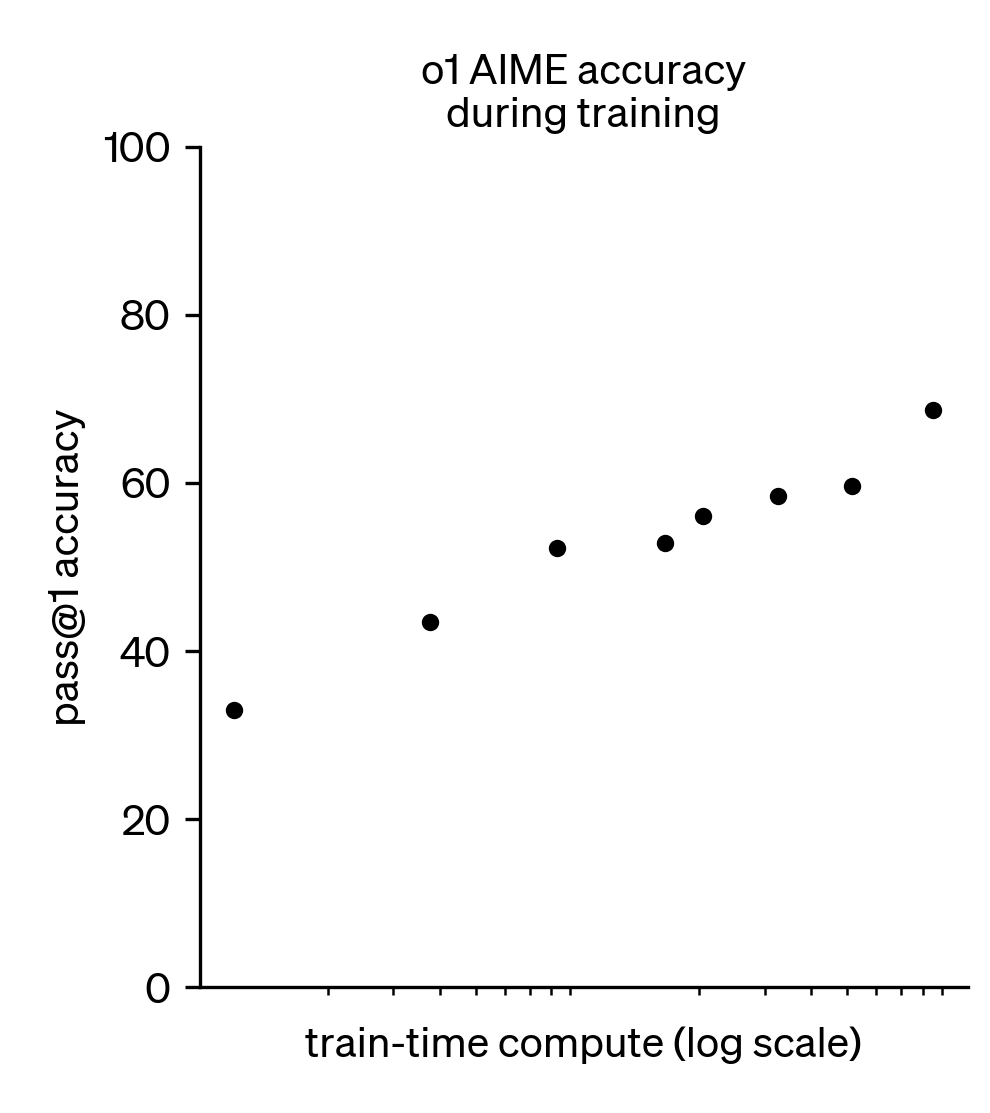
The scaling RL era
RL is now the load-bearing step in training the most capable models.
Reasoning models (o1, DeepSeek R1, etc.) are trained with these exact algorithms on verifiable rewards.
- Train-time compute scaling via RL
- Test-time compute scaling via extended reasoning
- RL went from “cherry on top” to a core capability driver
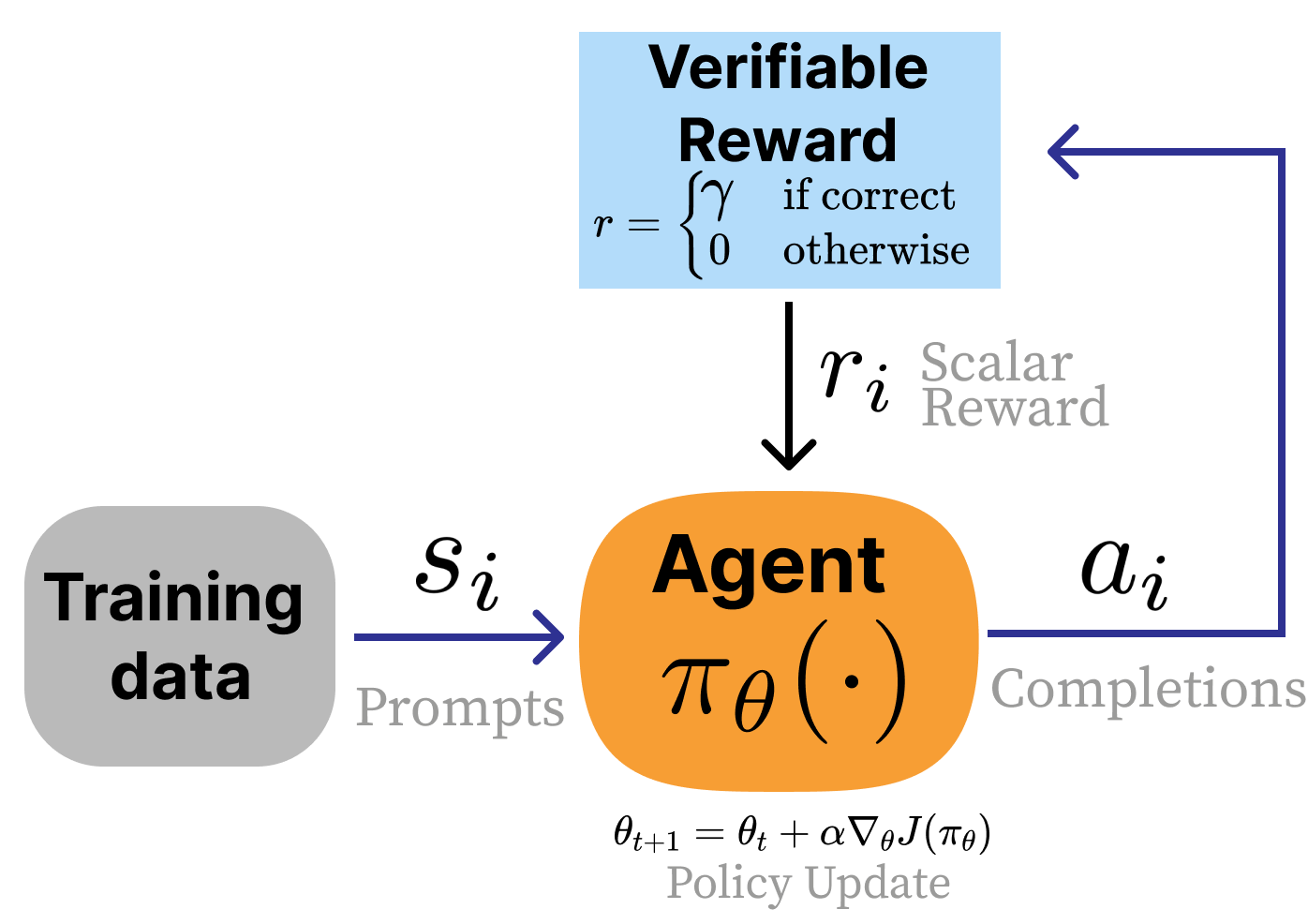
RLVR: Same algorithms, verifiable rewards
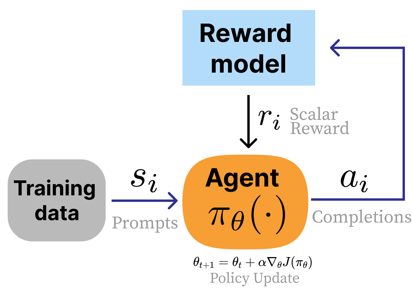
The RL methods in this lecture power both RLHF and RLVR:
- RLHF: reward model scores subjective quality
- RLVR: verification function checks correctness (math, code)
Same policy gradient algorithms, different reward source. We will cover tricks for reasoning training and a bunch of interesting models in depth in a future lecture.
Policy gradients: Core intuitions
Recall: Classical RL vs. RLHF
Classical RL: agent in an MDP (\mathcal{S}, \mathcal{A}, P, r, \gamma)
- Reward is a known function from the environment per step
- Optimize cumulative return: J(\pi) = \mathbb{E}_{\tau \sim p_\pi}\!\left[\sum_{t} \gamma^t r(s_t, a_t)\right]
RLHF: prompts from a dataset, no environment
- Reward is learned from human preferences
- Response-level reward, regularized with KL penalty
- J(\pi) = \mathbb{E}\left[ r_\theta(x, y) \right] - \beta \, D_{\text{KL}}\!\left(\pi \| \pi_{\text{ref}}\right)
Notation in this lecture
This lecture uses (s, a) notation from the reinforcement learning literature, where s denotes states and a denotes actions. In the language model context, you will often see (x, y) instead, where x is the prompt and y is the completion.
The (s, a) framing is more general — these algorithms were designed for sequential decision problems where actions are taken at each timestep. However, many RLHF implementations treat the entire completion as a single action, making the (x, y) notation equally valid.
Notation: r_t for per-step rewards, R(\tau) for trajectory returns, \rho_t for importance-sampling ratios. We reserve \rho for ratios to avoid confusion with rewards.
Language models as episodic MDPs
| MDP concept | Language model |
|---|---|
| State s_t | Prompt + tokens generated so far: (x, y_{<t}) |
| Action a_t | Next token y_t |
| Transition | Deterministic: append token to sequence |
| Policy \pi_\theta(a_t \mid s_t) | LM next-token distribution |
| Episode | One prompt → completion |
| Terminal reward | RM score or verifier output |
| \gamma | Typically 1.0 (no discounting) |
Two views of this MDP: token-level (each token is a separate action, used in PPO with GAE) vs. sequence-level (entire completion is one action, used in REINFORCE/GRPO).
What are we optimizing?
Choose policy parameters \theta that maximize reward on average under the current policy.
Let p_\theta(\tau) be the trajectory distribution induced by the current policy.
In practice, we estimate this expectation with sampled rollouts:
We craft a gradient/derivative that lets us optimize this.
How a policy gradient works
Make actions more likely when they lead to better outcomes.
Read it as two questions answered at once:
- \nabla_\theta \log \pi_\theta(a_t \mid s_t) — which action?
- \Psi_t — how good was it? A scalar scoring the outcome.
How a policy gradient works
Make actions more likely when they lead to better outcomes.
Read it as two questions answered at once:
- \nabla_\theta \log \pi_\theta(a_t \mid s_t) — which action? How each parameter influenced the probability of taking action a_t in state s_t. This connects the outcome back to the knobs that caused it.
- \Psi_t — how good was it? A scalar scoring the outcome. Positive means good, negative means bad, magnitude says how much.
An oversimplification (e.g. intuition in case of batch size of 1): the gradient is a vector with one entry per parameter. A positive entry means “increasing this parameter made the action more likely,” a negative entry means the opposite. In practice, the update averages over many such vectors — what survives is the net vote across the batch.
Multiply them: \Psi_t > 0 updates parameters to make a_t more likely, \Psi_t < 0 updates them to make it less likely.
The rest of this section is about choosing a smart \Psi_t — different choices (total return, advantage, TD residual) trade off variance and bias, but all plug into this same update.
The policy gradient equation
A preview of where we end up:
The core idea is that we sample over trials in the environment and estimate the gradient.
Where \Psi_t is the learning signal telling the optimizer how good the action was. The choice of \Psi_t determines the algorithm’s variance, bias, and compute cost.
Key RL quantities
Three quantities appear throughout this lecture:
Value function V(s): expected future return from state s
Action-value Q(s, a): expected return after taking action a in state s
Advantage A(s, a) = Q(s, a) - V(s): how much better is action a compared to average? Positive → reinforce, negative → suppress, zero → no update.
In RLHF: often \gamma = 1 (no discounting) because the unit of optimization is the full completion.
What \Psi_t can be
Popular choices for \Psi_t (rewards can also be discounted by \gamma):
| \Psi_t | Description | Variance | Bias | |
|---|---|---|---|---|
| 1. | R(\tau) = \sum_{t=0}^{T} r_t | Total trajectory reward | Highest | None |
| 2. | \sum_{t'=t}^{T} r_{t'} | Future return from t (the return, G_t) | High | None |
| 3. | G_t - b(s_t) | Baselined return | Lower | None |
| 4. | Q^{\pi}(s_t, a_t) | State-action value function | Med | Depends |
| 5. | A^{\pi}(s_t, a_t) = Q - V | Advantage function | Low (with good V) | None |
| 6. | r_t + \gamma V(s_{t+1}) - V(s_t) | TD residual | Low | Some |
A baseline b(s_t) is any value subtracted from the reward signal to reduce variance. We’ll show below that this does not change the expected gradient.
Deriving the policy gradient
Setup: Differentiating an expectation
Ideally, we want \nabla_\theta J(\theta), but we can’t do that (the state sampling distribution itself depends on \theta).
Written as an integral, the objective is:
Setup: Differentiating an expectation
Ideally, we want \nabla_\theta J(\theta), but we can’t do that (the state sampling distribution itself depends on \theta).
Written as an integral, the objective is:
Taking the gradient directly:
We can sample trajectories from p_\theta(\tau), but not from \nabla_\theta p_\theta(\tau), since it is not a probability distribution.
The derivation is a few key tricks to let us approximate or compute this.
Applying the idea of computing the gradient from trajectories
Substituting the log-derivative identity (more on this soon) into the gradient:
Now we can estimate this with Monte Carlo sampling!
Applying the idea of computing the gradient from trajectories
The only non-obvious step is the middle line:
This is the log-derivative identity, derived from the chain rule for \log.
It rewrites the gradient of a probability in terms of a log-probability, which is much easier to work with.
Applying the idea of computing the gradient from trajectories
Where did the p_\theta(\tau) term go?
It became the sampling distribution inside the expectation:
Monte Carlo then estimates that expectation by sampling trajectories from the policy:
So there is no explicit p_\theta(\tau_i) term in code: more likely trajectories already appear more often in the sampled batch.
At a high level, rollout generation handles the sampling, and the loss code handles R(\tau_i)\,\nabla_\theta \log p_\theta(\tau_i).
Expanding log probability of trajectory to compute \nabla_\theta
The trajectory probability factorizes:
Taking the log:
For language models, this is the familiar autoregressive pattern: a sequence log-probability becomes a sum of token log-probabilities.
Expanding log probability of trajectory to compute \nabla_\theta
Now take the gradient w.r.t. \theta:
- \nabla_\theta \log d_0(s_0) = 0 — initial state distribution doesn’t depend on \theta
- \nabla_\theta \log p(s_{t+1} \mid s_t, a_t) = 0 — environment dynamics don’t depend on \theta
- Only \nabla_\theta \log \pi_\theta(a_t \mid s_t) survives!
Expanding log probability of trajectory to compute \nabla_\theta
Now take the gradient w.r.t. \theta:
- \nabla_\theta \log d_0(s_0) = 0 — initial state distribution doesn’t depend on \theta
- \nabla_\theta \log p(s_{t+1} \mid s_t, a_t) = 0 — environment dynamics don’t depend on \theta
- Only \nabla_\theta \log \pi_\theta(a_t \mid s_t) survives!
In language-model code, this is why you repeatedly see:
seq_log_probs = (token_log_probs * completion_mask).sum(dim=-1)
loss = -(seq_log_probs * advantages).mean()
loss.backward()
Autodiff turns that summed log-probability into the corresponding sum of per-token gradients!
From full return to future rewards
An action at time t can’t affect past rewards. So instead of weighting by the full trajectory reward R(\tau):
We can replace R(\tau) with the return-to-go G_t = \sum_{t'=t}^{T} r_{t'} — only future rewards from t onward:
This doesn’t change the expected gradient, but removes noise from past rewards that the current action couldn’t have influenced. This is the step from \Psi_t option 1 → option 2 in our taxonomy.
Baselines keep the estimator unbiased
Raw returns are noisy. The same action can appear in trajectories with very different total rewards because of later sampled actions and, in classical RL, environment randomness.
The role of a baseline is to center that noisy signal: instead of asking “was the return high?”, we ask “was it higher or lower than expected for this state?”
Baselines keep the estimator unbiased
Raw returns are noisy. The same action can appear in trajectories with very different total rewards because of later sampled actions and, in classical RL, environment randomness.
The role of a baseline is to center that noisy signal: instead of asking “was the return high?”, we ask “was it higher or lower than expected for this state?”
Use a centered return:
where the baseline b(s_t) depends only on the state, not on which action was sampled.
Subtracting this baseline doesn’t change the expected gradient:
Baselines keep the estimator unbiased
Raw returns are noisy. The same action can appear in trajectories with very different total rewards because of later sampled actions and, in classical RL, environment randomness.
Use a centered return, \Psi_t = G_t - b(s_t).
Subtracting this baseline doesn’t change the expected gradient:
The first term is the original estimator. The second vanishes:
The gradient of a normalized distribution sums to zero — so we’re free to subtract any function of state as a baseline. This is why \Psi_t options 3–5 reduce variance without introducing bias.
Recall: What \Psi_t can be
Popular choices for \Psi_t (rewards can also be discounted by \gamma):
| \Psi_t | Description | Variance | Bias | |
|---|---|---|---|---|
| 1. | R(\tau) = \sum_{t=0}^{T} r_t | Total trajectory reward | Highest | None |
| 2. | \sum_{t'=t}^{T} r_{t'} | Future return from t (the return, G_t) | High | None |
| 3. | \sum_{t'=t}^{T} r_{t'} - b(s_t) | Baselined return | Lower | None |
| 4. | Q^{\pi}(s_t, a_t) | State-action value function | Med | Depends |
| 5. | A^{\pi}(s_t, a_t) = Q - V | Advantage function | Lowest | None |
| 6. | r_t + \gamma V(s_{t+1}) - V(s_t) | TD residual | Low | Some |
A baseline b(s_t) is any value subtracted from the reward signal to reduce variance — we’ll show why this is unbiased shortly.
The policy gradient estimator
Combining the log-derivative trick, return-to-go, and baseline subtraction:
This is the policy gradient theorem. Every algorithm in this lecture is an instantiation with a specific choice of \Psi_t and regularization.
For language models, this means the sum runs over generated tokens in the completion, while \Psi_t determines how each token is weighted.
Policy gradient derivation recap
- Log-derivative trick turns \nabla p_\theta(\tau) into a sampleable expectation
- Expanding \log p_\theta(\tau) gives a sum of policy log-prob terms
- \Psi_t is the learning signal: return, advantage, or TD-style estimate
- In code: sample rollouts, sum token log-probs, weight by \Psi_t, average
Wiring RLHF for language models
The RLHF training loop
Before diving into specific algorithms, let’s revisit the full RLHF setup they plug into.
The reference model
The reference model \pi_\text{ref} is a frozen copy of the policy at the start of RL training (typically the SFT checkpoint).
It serves one purpose: anchor the policy so it doesn’t drift too far during optimization.
Without it, the policy can exploit the reward model — finding high-scoring outputs that are degenerate or repetitive (reward hacking).
KL divergence as regularization
The KL penalty measures how far the current policy has drifted from the reference at each token:
In practice:
- Generate a completion from \pi_\theta
- Compute log-probs of those same tokens under both \pi_\theta and \pi_\text{ref}
- Subtract to get the per-token KL
The shaped reward becomes: \tilde{r}_t = -\beta \, \text{KL}_t for intermediate tokens, \tilde{r}_T = R(\tau) - \beta \, \text{KL}_T for the final token.
KL in RLHF vs. RLVR
RLHF (reward model signal): KL penalty is critical — the reward model is a learned proxy, and the policy will exploit any imperfections without regularization.
RLVR (verifiable rewards, e.g. math correctness): KL is often reduced or removed entirely. The reward is ground truth, so there’s less to exploit. Some RLVR setups (e.g. DeepSeek R1) drop the reference model altogether, saving memory.
The trend: as reward signals become more reliable, the need for KL regularization decreases.
Two “old” policies — don’t confuse them
| \pi_{\theta_\text{old}} | \pi_\text{ref} | |
|---|---|---|
| What | Policy at last rollout | Policy at start of RL training (SFT checkpoint) |
| Updates | Every batch (or every K steps) | Never (frozen) |
| Used for | Importance-sampling ratio \rho_t | KL penalty |
| If dropped | Must use 1 gradient step per batch (on-policy) | Risk of reward hacking |
In some implementations, “old logprobs” refers to the generation-time logprobs — the model has simply been updated since those logprobs were computed, not a separate model copy.
REINFORCE
REINFORCE
REINFORCE is the simplest instantiation of the policy gradient.
It is the Monte Carlo form of policy gradient: sample trajectories, compute their returns, and use those sampled returns to weight the log-prob gradients.
REINFORCE
REINFORCE is the simplest instantiation of the policy gradient.
It is the Monte Carlo form of policy gradient: sample trajectories, compute their returns, and use those sampled returns to weight the log-prob gradients.
The name is an acronym for “REward Increment = Nonnegative Factor X Offset Reinforcement X Characteristic Eligibility.”
Three components:
- Nonnegative factor (\alpha): the learning rate
- Offset reinforcement (G_t - b(s_t)): centered return for stability
- Characteristic eligibility (\nabla \log \pi): how to attribute learning per token
REINFORCE
REINFORCE is the simplest instantiation of the policy gradient.
It is the Monte Carlo form of policy gradient: sample trajectories, compute their returns, and use those sampled returns to weight the log-prob gradients.
The name is an acronym for “REward Increment = Nonnegative Factor X Offset Reinforcement X Characteristic Eligibility.”
Three components:
- Nonnegative factor (\alpha): the learning rate
- Offset reinforcement (G_t - b(s_t)): centered return for stability
- Characteristic eligibility (\nabla \log \pi): how to attribute learning per token
The update rule:
The baseline problem
Without a baseline, the gradient weights each action by its raw return G_t. This doesn’t tell you whether an action was better or worse than expected — just how good the overall outcome was.
The gradient is high variance because the raw return mixes the quality of the action with the quality of the state. A good action in a bad state and a bad action in a good state can produce similar returns.
The baseline solution
Subtracting a baseline b(s) centers the signal: now the gradient weight is (G_t - b), which answers “was this action better or worse than expected from this state?”
Because b(s) does not depend on which action was sampled, it factors out and cancels. The expected gradient is unchanged — but the variance drops dramatically.
REINFORCE with baseline
The full REINFORCE gradient:
Here, G_t - b(s_t) is already an advantage estimate: how much better the realized return was than expected from state s_t.
Common baselines:
- Average reward over the batch (simplest)
- Moving average of recent rewards
- Learned value function V_\phi(s) (optional — bridges to actor-critic methods)
Basic REINFORCE needs no critic — just Monte Carlo returns and a simple baseline. Adding a learned V_\phi can reduce variance further but introduces the complexity of training a second model (… and moves towards PPO).
REINFORCE architecture
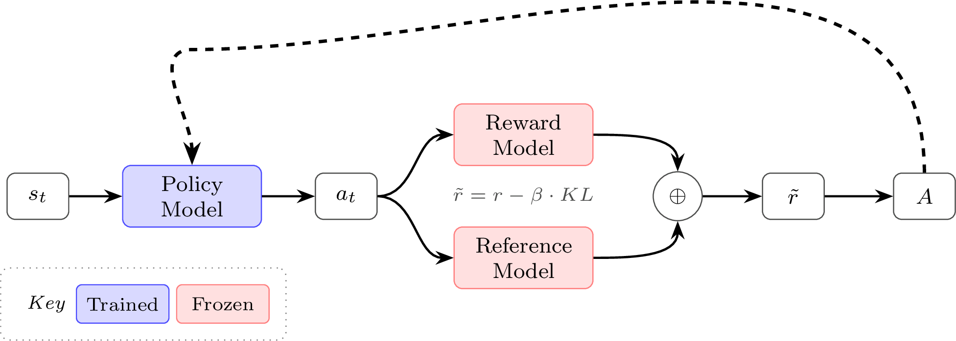
REINFORCE leave-one-out (RLOO)
RLOO: Leave-one-out baseline
Key idea: generate K completions per prompt. Use the other K-1 rewards as the baseline:
The advantage for completion k:
This is a per-prompt baseline that naturally captures prompt difficulty — hard prompts get low rewards across all completions, so the baseline is low.
Detail: Like REINFORCE without a critic, this same sequence-level advantage is broadcast to every token in the completion.
RLOO worked example
K = 4 completions for one prompt, with rewards [0.8, 0.3, 0.6, 0.5]:
| Completion | Reward | Baseline (avg of others) | Advantage |
|---|---|---|---|
| 1 | 0.8 | (0.3 + 0.6 + 0.5)/3 = 0.467 | +0.333 |
| 2 | 0.3 | (0.8 + 0.6 + 0.5)/3 = 0.633 | -0.333 |
| 3 | 0.6 | (0.8 + 0.3 + 0.5)/3 = 0.533 | +0.067 |
| 4 | 0.5 | (0.8 + 0.3 + 0.6)/3 = 0.567 | -0.067 |
Completion 1 (best) gets reinforced. Completion 2 (worst) gets suppressed. Completions 3 and 4 get small updates.
REINFORCE / RLOO summary
REINFORCE: Simplest policy gradient. Needs a baseline to reduce variance. No value function required.
RLOO: REINFORCE + a smart, per-prompt leave-one-out baseline. Multiple completions per prompt provide the baseline for free.
Both are the foundation for everything that follows:
- Linked intuitively to GRPO and other grouped-completion algorithms
- No value function needed (saves memory/compute)
- Simple to implement and debug
- Strong baselines in practice (Ahmadian et al., 2024) (Wang et al., 2024)
RLOO architecture
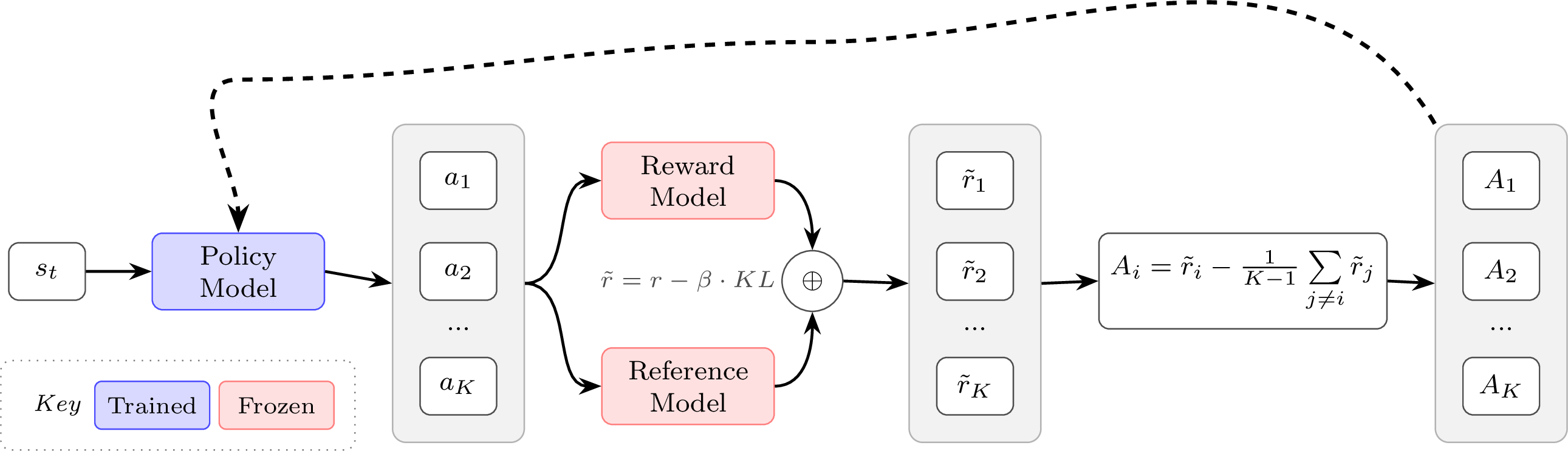
Proximal policy optimization (PPO)
If REINFORCE is so simple, why PPO?
All the algorithms in this lecture are on-policy: they generate fresh rollouts from the current policy each batch, then update on those rollouts. This is in contrast to off-policy RL methods (e.g. DQN) that store and replay old experience.
If REINFORCE is so simple, why PPO?
All the algorithms in this lecture are on-policy: they generate fresh rollouts from the current policy each batch, then update on those rollouts. This is in contrast to off-policy RL methods (e.g. DQN) that store and replay old experience.
The problem: vanilla policy gradient is sensitive to step size. Too large an update and the policy can collapse; too small and training is painfully slow. TRPO (Schulman et al., 2015) solved this with a hard trust-region constraint, but required expensive second-order optimization.
If REINFORCE is so simple, why PPO?
All the algorithms in this lecture are on-policy: they generate fresh rollouts from the current policy each batch, then update on those rollouts. This is in contrast to off-policy RL methods (e.g. DQN) that store and replay old experience.
The problem: vanilla policy gradient is sensitive to step size. Too large an update and the policy can collapse; too small and training is painfully slow. TRPO (Schulman et al., 2015) solved this with a hard trust-region constraint, but required expensive second-order optimization.
Proximal Policy Optimization (PPO) (Schulman et al., 2017) gets TRPO-like stability with a simple clipped objective — and because the clipping keeps updates conservative, you can safely take multiple gradient steps per batch of rollouts, improving sample efficiency.
What can we do with more conservative gradients?
Extract more signal from the batch! This introduces new problems:
- How do we constrain the updates over multiple gradient updates?
- How do we take the policy gradient if the data has drifted off-policy?
PPO core idea 1: Constrained updates
Large gradient steps can destroy the policy (instability, over-optimization, etc.)
The solution: trust regions — limit how far the policy can move in a single update.
PPO core idea 2: Importance sampling
We want to take multiple gradient steps on a batch, but the data came from an old policy \pi_{\theta_\text{old}}.
Define the importance sampling ratio:
- If \rho_t = 1: current and old policy agree on this action
- If \rho_t > 1: current policy assigns higher probability than old
- If \rho_t < 1: current policy assigns lower probability than old
This ratio reweights old-policy samples to estimate new-policy gradients. Plugging that ratio into the earlier policy-gradient form gives a surrogate objective we can optimize on old-policy data.
The surrogate objective
Using importance sampling, the policy gradient becomes:
Intermediate problem: without constraints, maximizing this can take arbitrarily large steps — the ratio \rho_t can diverge far from 1, making the estimate unreliable.
The PPO clipped objective (put pieces together)
PPO clips the ratio to prevent large updates — a practical surrogate inspired by trust-region ideas. The original paper (Schulman et al., 2017) calls this L^{CLIP}, but it’s an objective we maximize, so we use J:
Where \rho_t(\theta) = \frac{\pi_\theta(a_t \mid s_t)}{\pi_{\theta_\text{old}}(a_t \mid s_t)} is the importance-sampling ratio.
Where \varepsilon is typically 0.1–0.2. The \min selects the more conservative estimate.
Positive advantage (\hat{A}_t > 0)
The action is better than average at that state — we want to increase its likelihood. Three sub-cases:
-
\rho_t < 1 - \varepsilon: Action is less likely under new policy.
Objective: \rho_t \hat{A}_t — normal gradient, push probability up -
1 - \varepsilon \leq \rho_t \leq 1 + \varepsilon: Action is roughly equally likely.
Objective: \rho_t \hat{A}_t — normal gradient, push probability up -
\rho_t > 1 + \varepsilon: Action is already more likely under new policy.
Objective: (1+\varepsilon)\hat{A}_t — gradient is zero, no update needed (CLIPPED)
Note: on the first gradient step, \rho_t = 1 (policy hasn’t changed yet), so the ratio starts near 1 and cases 1/3 only arise on subsequent steps.
\rho_t(\theta) = \pi_\theta / \pi_{\theta_\text{old}} (policy ratio)
Negative advantage (\hat{A}_t < 0)
The action was worse than average at that state — we want to decrease its likelihood. Three sub-cases:
-
\rho_t < 1 - \varepsilon: Action is already less likely under new policy.
Objective: (1-\varepsilon)\hat{A}_t — gradient is zero, no update needed (CLIPPED) -
1 - \varepsilon \leq \rho_t \leq 1 + \varepsilon: Action is roughly equally likely.
Objective: \rho_t \hat{A}_t — normal gradient, push probability down -
\rho_t > 1 + \varepsilon: Action is more likely under new policy.
Objective: \rho_t \hat{A}_t — normal gradient, push probability down
Note: on the first gradient step, \rho_t = 1 (policy hasn’t changed yet), so the ratio starts near 1 and cases 1/3 only arise on subsequent steps.
\rho_t(\theta) = \pi_\theta / \pi_{\theta_\text{old}} (policy ratio)
Zero advantage (\hat{A}_t = 0)
The action was exactly as good as expected. The loss is zero — no update.
Clipping summary
In all cases, clipping stops the gradient when the policy has already moved enough in the right direction:
| Advantage | Within trust region | Outside trust region |
|---|---|---|
| \hat{A}_t > 0 | Normal gradient (reinforce) | Zero gradient if \rho_t > 1+\varepsilon |
| \hat{A}_t < 0 | Normal gradient (suppress) | Zero gradient if \rho_t < 1-\varepsilon |
| \hat{A}_t = 0 | No update | No update |
The clipping is one-sided per advantage sign: it caps movement when the policy has already moved enough in the beneficial direction, but never blocks correction in the detrimental direction.
PPO clipping visualized
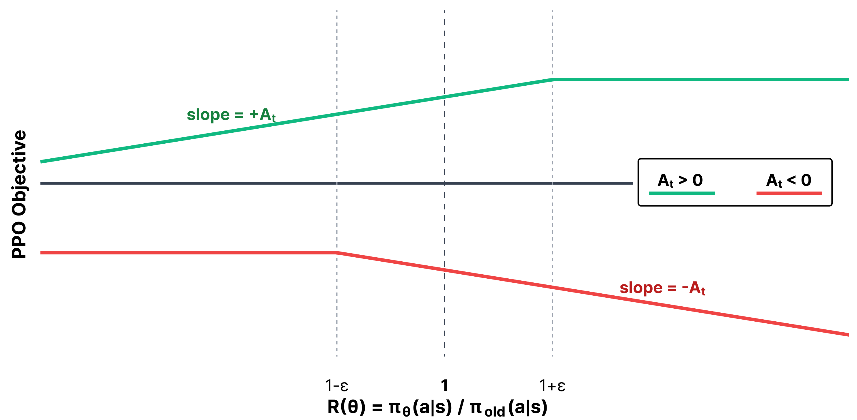
The value function (critic)
PPO trains a value function V_\phi(s) alongside the policy — the expected future return from state s_t:
- Separate parameters \phi (often initialized from the reward model or SFT model)
- Predicts post-KL shaped future return at each token position
- Trained via MSE against post-KL returns: \mathcal{L}_V = \frac{1}{2}(V_\phi(s_t) - G_t)^2
The value function serves as a learned baseline for advantage estimation.
How PPO-RLHF gets token-level credit
PPO-style RLHF often starts with one scalar reward for the whole completion. How does that become a per-token training signal?
- KL penalty shapes intermediate tokens: at each token t, subtract \beta \cdot \text{KL}_t from the reward → per-token reward signal
- Final token gets the RM score: r_T = R(\tau) - \beta \, \text{KL}_T, all other tokens get r_t = -\beta \, \text{KL}_t
- GAE propagates credit backward: the value function + TD residuals assign per-token advantages from these shaped rewards
This is how PPO-RLHF turns a sequence-level reward into token-level training.
Advantage estimation
The simplest advantage: \hat{A}_t = G_t - V_\phi(s_t)
Why advantages help:
- Centering reduces variance — we’re asking “how much better is this action than average?” rather than “how good was the total return?”
- Credit assignment — with per-token values, each token gets its own advantage signal
This Monte Carlo estimate is simple and unbiased, but it can be high variance. Temporal Difference (TD) methods and Generalized Advantage Estimation (GAE) trade some bias for lower variance.
The TD residual
The temporal difference (TD) residual measures how much the actual reward exceeded the value prediction:
This is the 1-step advantage estimate: low variance (uses learned V_\phi) but potentially high bias (if V_\phi is inaccurate).
GAE: K-step advantage
We can extend to K steps:
As k \to \infty, we recover the full Monte Carlo advantage G_t - V_\phi(s_t) (no bias, highest variance).
GAE: Exponential weighting
GAE uses an exponentially-weighted average across all K-step estimates:
Where \lambda \in [0, 1] controls the bias-variance tradeoff.
GAE: Bias-variance tradeoff
| \lambda | Behavior | Variance | Bias |
|---|---|---|---|
| 0 | Pure TD (1-step) | Lowest | Highest |
| 0.95 | Typical default for LLMs | Balanced | Balanced |
| 1 | Monte Carlo advantage | Highest | None |
The \gamma here is typically 1.0 for language models (no discounting). These rankings assume an accurate V_\phi — in practice, a poorly trained critic can make even low-\lambda estimates unreliable.
PPO-RLHF: Full policy objective
A schematic high-level view of PPO-RLHF combines the clipped PPO objective with a KL regularizer:
Two layers of regularization:
- Clipping — limits how far the policy moves per batch (trust region)
- KL penalty — limits total drift from the reference policy across training
These serve different purposes and are not redundant.
PPO training loop (conceptual)
The PPO training loop:
- Generate: sample prompts, generate completions with current policy \pi_\theta
- Score: compute rewards with reward model + KL penalty from \pi_\text{ref}
- Estimate advantages: compute GAE using learned value function V_\phi
- Update (K epochs): clipped policy gradient + value function loss on the same batch
- Repeat: new batch, sync \pi_{\theta_\text{old}} \leftarrow \pi_\theta
Typical: K = 2–4 gradient steps per batch before re-generating.
PPO: Four models in memory
PPO requires four models:
| Model | Purpose | Updates? |
|---|---|---|
| Policy \pi_\theta | Generates completions | Yes |
| Value function V_\phi | Estimates per-token expected return | Yes |
| Reference policy \pi_\text{ref} | KL penalty anchor | Frozen |
| Reward model r_\psi | Scores completions | Frozen |
This is memory-intensive — a key motivation for simpler alternatives like GRPO.
PPO architecture
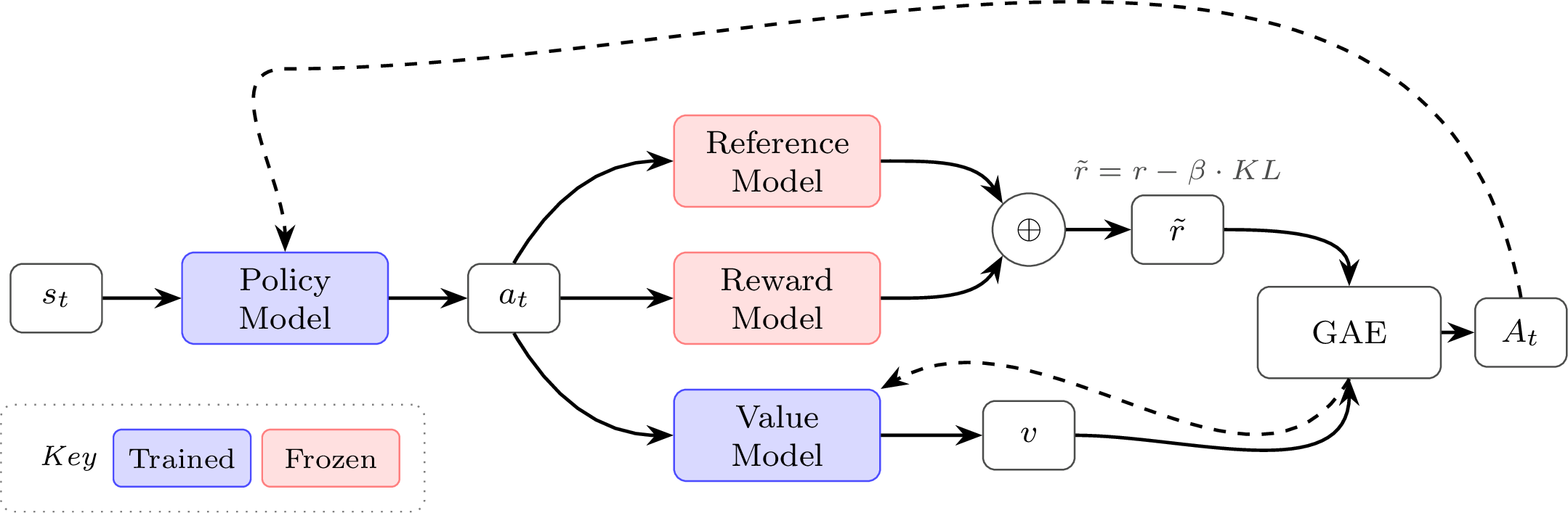
GRPO & modern variants
GRPO: PPO for the reasoning era
Group Relative Policy Optimization (GRPO) was introduced in DeepSeekMath (Shao et al., 2024) for math reasoning and has since become the go-to algorithm for RL on language models. It keeps PPO’s clipped objective but drops the value function entirely.
Core idea: generate G completions per prompt, use the group’s reward statistics as the baseline — no learned critic needed.
- Simpler to implement and debug than PPO
- Saves memory (one fewer model copy)
- Natural fit for RLVR where you have a clear verification signal and higher variance rewards (e.g. 0 or 1 for correctness)
- Popularized with DeepSeek R1 and everything that followed
GRPO advantage
For a group of G completions with rewards R_1, \ldots, R_G:
Z-score normalization: positive advantage for above-average completions, negative for below.
Each token in completion i gets the same advantage (sequence-level, not per-token).
GRPO objective
Clipped ratio (like PPO) + group-normalized advantages + KL penalty directly in loss:
Where the clipping applies per-token: \rho_{i,t} = \frac{\pi_\theta(a_{i,t} \mid s_t)}{\pi_{\theta_\text{old}}(a_{i,t} \mid s_t)}, but \hat{A}_i is shared across all tokens in the completion (sequence-level advantage, per-token ratio).
GRPO vs PPO
| PPO | GRPO | |
|---|---|---|
| Value function | Learned V_\phi | None |
| Advantage | Per-token via GAE | Sequence-level, group z-score |
| KL penalty | In reward (before advantages) | In loss (default, but optional) |
| Models in memory | 4 (policy, value, ref, RM) | 3 (policy, ref, RM) or 2 without KL |
| Complexity | Higher | Lower |
| Popular for | General RLHF | Reasoning / RLVR (DeepSeek R1) |
GRPO is PPO minus the value function, with a statistical baseline instead.
RLOO vs GRPO
Both use multiple completions per prompt. The key difference is in the PPO-style clipping for GRPO:
| RLOO | GRPO | |
|---|---|---|
| Baseline | Leave-one-out mean | Group mean (z-scored) |
| Update style | REINFORCE (no clipping) | PPO-style clipped ratio |
| KL penalty | Optional (in reward) | In loss (default, but optional) |
| Advantage | R_k - \frac{1}{K-1}\sum_{j \neq k} R_j | \frac{R_i - \text{mean}}{\text{std}} |
Same principle (compare to peers), different mechanics. Without std normalization, the GRPO-style advantage estimate becomes equivalent to RLOO up to a scaling constant.
GSPO: Sequence-level ratios
Problem: aggregating per-token importance ratios across long sequences is numerically unstable. A single token with a large ratio can dominate the update.
GSPO uses a geometric mean — a single, length-normalized importance weight per response:
The geometric mean stays in a reasonable numerical range for any sequence length — similar gradient signal, better numerics. The full objective mirrors GRPO but with the sequence-level ratio:
The clipping range \varepsilon now operates on a per-token average scale, making it comparable across different completion lengths.
CISPO: Clipped importance sampling
CISPO clips the importance weights themselves rather than the objective, using a stop-gradient:
Key difference from PPO: every token still receives a gradient signal — the weight just bounds how much it’s amplified. Asymmetric bounds (\varepsilon^{+} > \varepsilon^{-}) allow more aggressive reward-increasing updates, encouraging exploration.
GRPO architecture
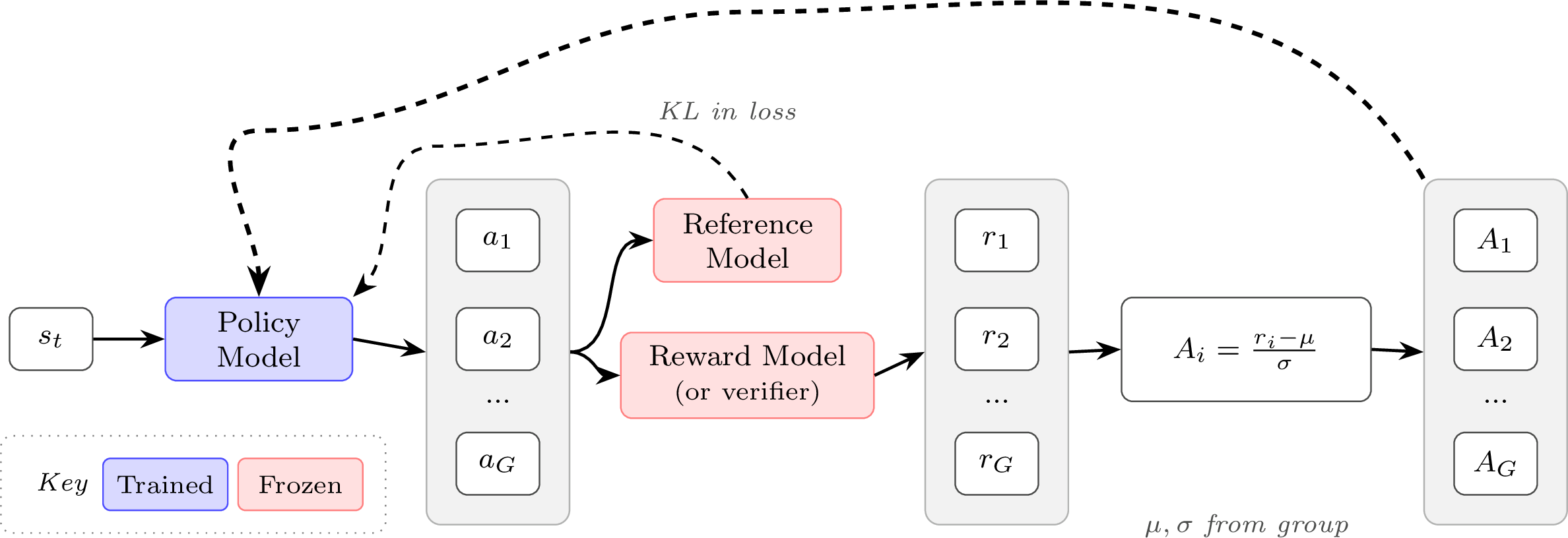
Conclusion
Lecture summary
In most RLHF setups, data quality and reward signal quality dominate; algorithm choice mostly determines stability, efficiency, and engineering burden. All methods optimize the same policy gradient objective:
They differ in:
- What \Psi_t is: total return, advantage, group-normalized advantage
- How updates are bounded: no clipping (REINFORCE), objective clipping (PPO/GRPO), weight clipping (CISPO)
- Memory and compute: 2–4 models, value function training or not
RL cheatsheet
A one-page reference of all core RL loss functions is available at:
Next lecture: RL implementation
Lecture 4 turns these algorithms into working code:
- Core loss implementations: Setting up RL algorithms with language models
- Loss aggregation: per-sequence vs per-token normalization and why it matters
- Infra setup: what to store (log-probs, values, ref log-probs) and what goes wrong when you don’t
- Trade-offs: monitoring training, identifying reward hacking, fixing common failures