Lecture 6: Direct Preference Optimization
Nathan Lambert
Post-training course. Chapter 8 on Direct Alignment Algorithms.
Why DPO was – and is – such a big deal
The Direct Preference Optimization paper (Rafailov et al., 2023) was a breakthrough in the accessibility of RLHF and post-training research. Some context:
- DPO paper was released in May of 2023, when many groups were struggling to get open-source replications of RLHF pipelines going. Most “aligned” models were just SFT.
- It took until about the fall of 2023 for people to figure out the right data and settings for DPO to work
- Zephyr-Beta, Tülu 2, and other models that fall opened the floodgates of post-training research. Iterating on DPO methods in 2024 felt as exciting as RL methods in 2025 or tool-use methods in 2026.
- Terminology note: I call the class of algorithms that operate like DPO on static preference data Direct Alignment Algorithms (DAAs). The name didn’t stick much, but we’ll see there are a ton of variants!
The DPO debate (DPO v RL)
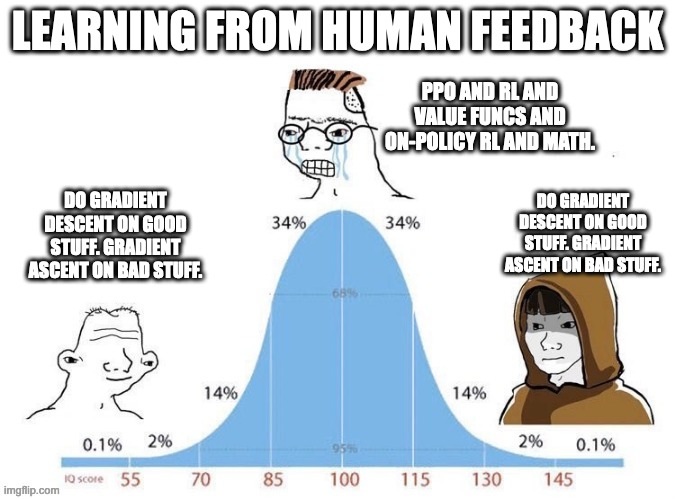
This lecture
We will derive Direct Preference Optimization (DPO) from scratch, then look at how it is used in practice.
The promise of DPO:
- No separate reward model
- No reinforcement learning loop
- Just a single, directly-differentiable loss on preference pairs
The plan, in four steps:
- Solve the RLHF objective for its optimal policy
- Invert that to write the reward in terms of the policy
- Plug it into the Bradley-Terry preference model
- Read off the DPO loss and its gradient
Rafailov et al., 2023 — “Your Language Model is Secretly a Reward Model” (Rafailov et al., 2023).
Recall: Where DPO sits in the pipeline
Classic RLHF is three moving parts:
- Collect human preference pairs
- Train a reward model r_\phi(x,y)
- Optimize the policy against r_\phi with RL (e.g. PPO), under a KL penalty
DPO collapses steps 2 and 3 into one supervised-style loss.
The key realization we will prove:
The optimal RLHF policy and the reward model are two views of the same object. If we know one, we know the other in closed form.
So we can train the policy directly on preferences.
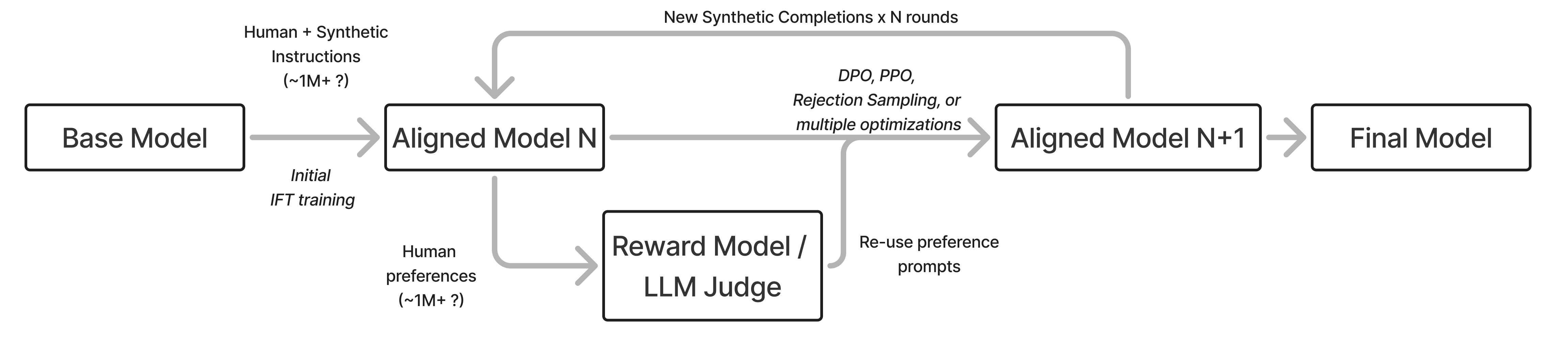
DPO at a glance: Where we’re headed
The whole derivation lands on two objects.
Optimal policy — the RLHF solution in closed form:
DPO loss — what you actually train:
In practice, that loss is just a few lines:
pi_logratios  = policy_chosen_logps  - policy_rejected_logps
ref_logratios = reference_chosen_logps - reference_rejected_logps
logits = pi_logratios - ref_logratios
losses = -F.logsigmoid(beta * logits)
Everything between here and the implementation is why this is the right loss.
DPO derivation P1/4: Deriving the optimal policy
Start with the RLHF optimization problem
We want to find the \pi that solves this equation! But, without RL.
Fold the KL into the expectation
Fold the KL into the expectation
Flip to a minimization & clean-up
Flip to a minimization & clean-up
Flip to a minimization & clean-up
Fold the optimization target into one log-ratio
Pick up where we left off and fold the bracket into a single log-ratio, using \tfrac{1}{\beta} r = \log e^{\,r/\beta}:
- \pi is now measured against \pi_{\text{ref}}\,e^{r/\beta}: the reference reweighted by reward — each response’s probability is multiplied by e^{r/\beta}, which is larger the higher its reward (\beta sets how aggressive the reweighting is).
- If that target were a probability distribution q, this \min_{\pi} would be a KL divergence, \mathbb{E}_{y\sim\pi}\!\big[\log\tfrac{\pi}{q}\big] = \mathcal{D}_{\text{KL}}(\pi\,\|\,q) — minimized exactly, in closed form (Gibbs’ inequality).
Introduce the partition function Z(x)
We are minimizing \min_{\pi}\ \mathbb{E}_{y\sim\pi}\Big[\, \log\frac{\pi(y\mid x)}{\pi_{\text{ref}}(y\mid x)\,e^{\,r(x,y)/\beta}} \,\Big].
Why do we want \pi to match that denominator?
Introduce the partition function Z(x)
We are minimizing \min_{\pi}\ \mathbb{E}_{y\sim\pi}\Big[\, \log\frac{\pi(y\mid x)}{\pi_{\text{ref}}(y\mid x)\,e^{\,r(x,y)/\beta}} \,\Big].
Why do we want \pi to match that denominator? Because \mathbb{E}_{y\sim\pi}\big[\log\tfrac{\pi}{q}\big] is a KL divergence \mathcal{D}_{\text{KL}}(\pi\,\|\,q) — it is \ge 0, and equals 0 only when \pi = q. So the minimizer is whatever distribution q sits in the denominator.
Introduce the partition function Z(x)
We are minimizing \min_{\pi}\ \mathbb{E}_{y\sim\pi}\Big[\, \log\frac{\pi(y\mid x)}{\pi_{\text{ref}}(y\mid x)\,e^{\,r(x,y)/\beta}} \,\Big].
Why do we want \pi to match that denominator? Because \mathbb{E}_{y\sim\pi}\big[\log\tfrac{\pi}{q}\big] is a KL divergence \mathcal{D}_{\text{KL}}(\pi\,\|\,q) — it is \ge 0, and equals 0 only when \pi = q. So the minimizer is whatever distribution q sits in the denominator.
The catch: our denominator \pi_{\text{ref}}\,e^{r/\beta} is not a distribution — summed over y it does not equal 1.
Introduce the partition function Z(x)
We are minimizing \min_{\pi}\ \mathbb{E}_{y\sim\pi}\Big[\, \log\frac{\pi(y\mid x)}{\pi_{\text{ref}}(y\mid x)\,e^{\,r(x,y)/\beta}} \,\Big].
Why do we want \pi to match that denominator? Because \mathbb{E}_{y\sim\pi}\big[\log\tfrac{\pi}{q}\big] is a KL divergence \mathcal{D}_{\text{KL}}(\pi\,\|\,q) — it is \ge 0, and equals 0 only when \pi = q. So the minimizer is whatever distribution q sits in the denominator.
The catch: our denominator \pi_{\text{ref}}\,e^{r/\beta} is not a distribution — summed over y it does not equal 1. We normalize it with the partition function:
- Now q(y\mid x) = \tfrac{1}{Z(x)}\,\pi_{\text{ref}}(y\mid x)\,e^{\,r/\beta} is a valid distribution.
- The objective becomes a genuine \mathcal{D}_{\text{KL}}(\pi\,\|\,q) — minimized exactly at \pi = q (made rigorous with Gibbs’ inequality shortly).
- Next we massage the inside of the objective so Z(x) appears.
Revisiting the objective with the partition function Z(x)
Revisiting the objective with the partition function Z(x)
Revisiting the objective with the partition function Z(x)
Revisiting the objective with the partition function Z(x)
Turn the objective into a KL divergence
Fold \tfrac{1}{\beta} r = \log e^{\,r/\beta} into the denominator of the first term in the objective (again, log rules) and name it q(y\mid x) = \tfrac{1}{Z(x)}\,\pi_{\text{ref}}(y\mid x)\,e^{\,r(x,y)/\beta} — a valid distribution over y. The objective is:
\log Z(x) does not depend on y, so pull it out of the inner expectation:
The inner expectation is exactly a KL divergence, \mathbb{E}_{y\sim\pi}\big[\log\tfrac{\pi}{q}\big] = \mathcal{D}_{\text{KL}}(\pi\,\|\,q):
Apply Gibbs’ inequality to read off \pi^{*}
Where we landed – the objective is now a KL plus a \pi-independent constant:
- \log Z(x) does not depend on \pi — only the KL term can be optimized.
- A KL is \ge 0 and equals 0 only when \pi = q (Gibbs’ inequality), so the minimizer is \pi^{*} = q:
DPO derivation P2/4: Recovering the reward from the policy (needed to implement it)
Invert \pi^{*} for the implicit reward
Invert \pi^{*} for the implicit reward
Invert \pi^{*} for the implicit reward
Invert \pi^{*} for the implicit reward
Invert \pi^{*} for the implicit reward
DPO derivation P3/4: Connecting to Bradley-Terry preference (what our alignment data has looked like)
Recall the Bradley-Terry model
A preference between two responses is a softmax over their rewards:
Now substitute the implicit reward r^{*}(x,y) = \beta \log \tfrac{\pi^{*}(y\mid x)}{\pi_{\text{ref}}(y\mid x)} + \beta \log Z(x).
New here? See Lecture 2 and Chapter 5: Reward Modeling for the Bradley-Terry model.
Substitute the reward, then cancel Z(x)
- Every term carries the same factor \exp(\beta \log Z(x)) = Z(x)^{\beta}.
- Decompose e^{a+b}=e^a e^b and cancel the shared Z(x)^{\beta} — the intractable term is gone.
Divide through to a sigmoid
Write \Delta_i = \beta \log \tfrac{\pi^{*}(y_i\mid x)}{\pi_{\text{ref}}(y_i\mid x)}, so the cancelled form is p^{*} = \dfrac{e^{\Delta_1}}{e^{\Delta_1} + e^{\Delta_2}}. Multiply numerator and denominator by e^{-\Delta_1}:
- The numerator becomes 1; the denominator holds an exponential of the difference \Delta_2 - \Delta_1.
With \sigma(z) = \tfrac{1}{1+e^{-z}}, this is a sigmoid (\Delta_i = \beta \log \tfrac{\pi^{*}(y_i\mid x)}{\pi_{\text{ref}}(y_i\mid x)}):
- A sigmoid of the difference of two log-ratios — Bradley-Terry, with the policy in place of the reward model.
DPO derivation P4/4: The loss function and gradient
The DPO loss
Minimize the negative log-likelihood of the observed preferences (y_c \succ y_r) – this is making the probability more likely:
Plug in the sigmoid form of p, with the trainable policy \pi_{\theta} as the implicit reward:
This is directly differentiable — no reward model, no sampling, no RL loop.
The DPO gradient
Start by taking the gradient of the previous loss function.
Let u = \big(\beta \log \tfrac{\pi_{\theta}(y_c\mid x)}{\pi_{\text{ref}}(y_c\mid x)} - \beta \log \tfrac{\pi_{\theta}(y_r\mid x)}{\pi_{\text{ref}}(y_r\mid x)}\big) — the term inside \sigma.
Chain rule, starting with \tfrac{d}{dz}\log\sigma(z) = \tfrac{\sigma'(z)}{\sigma(z)} as the inner operation:
Substitute \sigma'(u) = \sigma(u)\big(1-\sigma(u)\big) and cancel \sigma(u):
The DPO gradient
The reflection identity 1-\sigma(u) = \sigma(-u) flips the argument, giving the compact form:
Now differentiate u, where -u = \beta\log\tfrac{\pi_{\theta}(y_r\mid x)}{\pi_{\text{ref}}(y_r\mid x)} - \beta\log\tfrac{\pi_{\theta}(y_c\mid x)}{\pi_{\text{ref}}(y_c\mid x)}. Only \pi_{\theta} depends on \theta — \pi_{\text{ref}} is frozen, so its \log terms drop:
Substitute \nabla_{\theta} u and write \sigma(-u) out in full:
The DPO gradient
- Weight w \in (0,1) is larger when the model is more wrong — when it ranks the rejected response above the chosen the loss is higher.
- The delta-gradient bracket raises the likelihood of y_c and lowers that of y_r.
- \beta scales the step, trading correct ordering against drift from \pi_{\text{ref}} (downstream of the KL penalty in the RLHF objective).
Recap: The DPO derivation
The reward model never had to be built — it was hiding inside the policy the whole time.
DPO weaknesses, variants, and implementation details
A subtle risk: The chosen probability can fall
The DPO loss only cares about the margin between the chosen and rejected log-ratios — not their absolute values. So the model can lower the loss by pushing the rejected probability down faster than the chosen, even while the chosen probability also falls.
Mediated through the partition function Z(x) in the derivation.
- Called likelihood displacement (Razin et al., 2025) (Ren & Sutherland, 2025); posited to push probability toward unaddressed, off-distribution behaviors.
- A reason some practitioners add an SFT term on the chosen response, or use fixes like Cal-DPO (Xiao et al., 2024) / AlphaPO (Gupta et al., 2025).
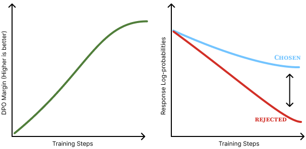
In a real run: Olmo 1B DPO — the chosen/rejected reward margin widens, yet the chosen log-prob itself can still drift down.
The \beta parameter and the static KL
\beta sets the strength of the KL constraint relative to reward maximization:
- Large \beta → policy stays close to \pi_{\text{ref}}; it barely moves.
- Small \beta → policy is free to deviate; it can over-optimize.
Crucially, DPO’s final KL distance is static: it steps directly to the optimal solution implied by the dataset and the chosen \beta. Online RL instead takes steps based on freshly sampled batches and a per-sample KL penalty. Some RL runs even include dynamically adjusted KL controllers.
A zoo of direct alignment algorithms
Each variant tweaks the loss to fix a limitation — often a one-line change. I started calling all the variants Direct Alignment Algorithms (DAAs). Two to start:
- Identity Preference Optimization (IPO) (Azar et al., 2024) — softens the preference probability away from Bradley-Terry to curb overfitting.
- Conservative DPO (cDPO) (Rafailov et al., 2023) (in the original DPO paper) — assumes the preference labels are noisy (flipped with probability \varepsilon) and softens the loss target accordingly.
- Offset DPO (ODPO) (Amini et al., 2024) — requires the chosen to beat the rejected by a margin offset, scaled by how strong the preference is.
A zoo of direct alignment algorithms
Two more that drop the reference model entirely:
- Odds Ratio Preference Optimization (ORPO) (Hong et al., 2024) — adds an odds-ratio pull toward the chosen response, folded directly into the SFT loss. The odds ratio uses only \pi_\theta, which allows dropping the reference model.
- Simple Preference Optimization (SimPO) (Meng et al., 2025) — length-normalizes the reward into an average log-prob, with a target margin \gamma. \tfrac{1}{|y|} normalizes by length; \gamma is a target margin; no \pi_{\text{ref}}.
The algorithm matters far less than the base model and the data. Still, many papers continued to make minor algorithmic tweaks. Many more exist than were on these slides.
Implementation is genuinely simple
No generation during training, no separate reward model — the heart of the loss is a few lines:
# log-prob gaps for policy and frozen reference
pi_logratios  = policy_chosen_logps - policy_rejected_logps
ref_logratios = reference_chosen_logps - reference_rejected_logps

# positive when policy shifts mass toward the chosen completion
logits = pi_logratios - ref_logratios
losses = -F.logsigmoid(beta * logits)
Tip: \pi_{\text{ref}} is frozen, so precompute and cache its log-probs to cut peak memory ~50%. Reference code: code/direct_alignment/.
DAAs work with synthetic preference data
These algorithms need feedback data, not necessarily human feedback data — AI feedback works just as well.
- Most modern DPO uses preferences labeled by a strong model. UltraFeedback (Cui et al., 2023) was the first prominent open synthetic preference dataset and helped kickstart the DPO era; Tülu 3 (Lambert et al., 2024), SmolLM 2 (Ben Allal et al., 2025), and others followed with larger synthetic-feedback recipes.
- On-policy data (some completions from the model you are tuning) helps the contrastive loss optimize the right token space within a complex post-training recipe (studied this specifically in Tülu 3).
- Delta Learning (Geng et al., 2025): later work argues the gap between chosen and rejected matters more than which models produced them (e.g. Qwen3-32B chosen vs Qwen3-0.6B rejected). Used this in Olmo 3!
DPO vs. RL: Offline vs. online
DPO and other DAAs
- Train on a fixed dataset collected ahead of time.
- Simpler, more stable, fast to iterate on data.
- Limited by the coverage of that dataset — a slightly lower performance ceiling.
PPO / policy gradient is online
- Generate fresh completions during training, score with a reward model.
- Can explore new regions → often higher peak performance (Ivison et al., 2024) (Xu et al., 2024) (Tajwar et al., 2024).
- More compute, more moving parts (four models in memory), more engineering complexity.
Where does this leave us today?
If so many models have used DPO well and it’s so simple, why does it seem like it comes up so infrequently – especially at the frontier?
Hypotheses for DPO’s role today
- Olmo 3 (Nov 2025) / SmolLM 3 (Jul 2025) – used DPO over reasoning traces after SFT to boost performance in a simple pipeline.
- NVIDIA Nemotron 3 (Dec 2025) – Mixed Preference Optimization: DPO + Binary Classifier Optimization in one offline stage, over data scored by a generative reward model.
- Liquid AI LFM2 (Nov 2025) – length-normalized DPO on semi-online data, before a final RLVR pass.
Hypotheses for DPO’s role today
- Olmo 3 (Nov 2025) / SmolLM 3 (Jul 2025) – used DPO over reasoning traces after SFT to boost performance in a simple pipeline.
- NVIDIA Nemotron 3 (Dec 2025) – Mixed Preference Optimization: DPO + Binary Classifier Optimization in one offline stage, over data scored by a generative reward model.
- Liquid AI LFM2 (Nov 2025) – length-normalized DPO on semi-online data, before a final RLVR pass.
How I see things:
- DPO works well in wonky, distillation-heavy recipes like Olmo – e.g. a model with a spikier distribution, with training data from many teacher models.
- DPO still works in other settings, but most labs have the engineering resources to do other things with higher peak performance.
- TLDR: DPO is a path to a good/solid model, but not to the best model. And DPO may do less in cleaner training recipes.