Q&A 2: Advanced derivation fixes, resources to go further, and notation gotchas

rlhfbook.com/course

Nathan Lambert

Corrections and reader questions from the GitHub, Discord, and YouTube comments. Lectures 5-7-ish.

Math corrections!

Correction: the KD-as-RL-advantage slide (Lecture 7)

A sharp-eyed viewer flagged the “KD as an RL advantage” slide:

The slide is missing a \pi_\theta(a_t \mid s_t) multiplier for A_t^{\mathrm{OPD}} (since it’s for a single token, else it would be the expectation). Also, the negative reverse-KL on the top line looks like the forward-KL on the second line, which can be confusing.

What the slide showed:

A_t^{\mathrm{OPD}} = -D_{\mathrm{KL}}\!\left(\pi_\theta(\cdot \mid s_t) \,\|\, \pi_T(\cdot \mid s_t)\right) \;{\color{red}\boxed{\color{red}=}}\; -\left(\log \pi_\theta(a_t \mid s_t) - \log \pi_T(a_t \mid s_t)\right)

A_t^{\mathrm{OPD}} = \log \pi_T(a_t \mid s_t) - \log \pi_\theta(a_t \mid s_t)

Source: viewer feedback on Lecture 7

Correction: the KD-as-RL-advantage slide (Lecture 7)

The reverse KL at state s_t is an expectation over student-sampled tokens:

D_{\mathrm{KL}}\!\left(\pi_\theta(\cdot \mid s_t) \,\|\, \pi_T(\cdot \mid s_t)\right) = \mathbb{E}_{a_t \sim \pi_\theta(\cdot \mid s_t)}\!\left[\log \pi_\theta(a_t \mid s_t) - \log \pi_T(a_t \mid s_t)\right]

You never sum over the vocabulary: the single sampled token is an unbiased estimate \hat{D}_{\mathrm{KL}} of that KL, and the advantage is its negative:

A_t^{\mathrm{OPD}} = -\hat{D}_{\mathrm{KL}} = -\left(\log \pi_\theta(a_t \mid s_t) - \log \pi_T(a_t \mid s_t)\right) = \log \pi_T(a_t \mid s_t) - \log \pi_\theta(a_t \mid s_t)

The old slide wrote a hard “=” to the full D_{\mathrm{KL}}; it’s an estimate, equal only in expectation.
Same form, opposite KL: \log \pi_T - \log \pi_\theta looks like forward KL – it’s reverse because we sample a_t \sim \pi_\theta (the student).
Fixed slide + details: Lecture 7 deck · PR #459.

Sources: (Lu & Thinking Machines Lab, 2025), (Schulman, 2020)

Correction: KL divergence is not a “distance” (Lecture 0)

I called the KL divergence a “distance” a few times. A viewer rightly pushed back:

KL is asymmetric (D_{\mathrm{KL}}(P\|Q)\neq D_{\mathrm{KL}}(Q\|P)) and violates the triangle inequality — so it is not a metric.

Fair — and I battled my editors on this too. In post-training teams “KL distance” is common colloquial shorthand as “how much has the model changed,” but technically it is a divergence.

For reference, some information theory:

D_{\mathrm{KL}}(P\|Q) = H(P,Q) - H(P) \ge 0

H(P) = the minimum expected code length for data from P; H(P,Q) = the cost of encoding it with a code built for Q.
No code beats the one matched to the true P, so H(P,Q)\ge H(P) — hence KL \ge 0. It measures extra coding cost, not a symmetric distance.

Source: viewer feedback on Lecture 0

Reading: how to estimate KL in practice

In RL we rarely compute the exact KL — we estimate it from sampled tokens. John Schulman’s note on the k_1 / k_2 / k_3 estimators (which is low-variance, which stays positive) is essential lore for anyone touching a KL penalty:

→ joschu.net/blog/kl-approx.html

Correction: the Bradley-Terry loss derivation (Lecture 2 / Ch 5)

What the slide showed: the full derivation

The reward model maximizes the Bradley-Terry preference probability, then manipulates it into the loss (all for a single example (x, y_c, y_r)):

\begin{aligned} \theta^* &= \arg\max_\theta \; P(y_c > y_r \mid x) && \text{the (wrong) setup: maximize per-example probability} \\[4pt] &= \arg\max_\theta \; \frac{\exp(r_\theta(y_c \mid x))}{\exp(r_\theta(y_c \mid x)) + \exp(r_\theta(y_r \mid x))} && \text{Bradley-Terry form} \\[4pt] &= \arg\max_\theta \; \frac{1}{1 + \exp\!\left(r_\theta(y_r \mid x) - r_\theta(y_c \mid x)\right)} && \text{divide through by } \exp(r_\theta(y_c \mid x)) \\[4pt] &= \arg\max_\theta \; \sigma\!\left(r_\theta(y_c \mid x) - r_\theta(y_r \mid x)\right) && \text{recognize } \sigma(z) = \tfrac{1}{1+e^{-z}} \\[4pt] &= \arg\max_\theta \; \log \sigma(\Delta) && \log \text{ is monotonic},\;\; \Delta = r_\theta(y_c \mid x) - r_\theta(y_r \mid x) \\[4pt] \Rightarrow\quad \mathcal{L}(\theta) &= -\log \sigma(\Delta) && \text{flip sign: maximization} \to \text{loss} \end{aligned}

Clean per-example — but training is over a dataset. Where does the average go?

Correction: the Bradley-Terry loss derivation (Lecture 2 / Ch 5)

A reader noted the reward-model derivation maximizes the per-example preference probability, then converts straight to the -\log\sigma loss (writing \Delta = r_\theta(y_c \mid x) - r_\theta(y_r \mid x)):

\theta^* = \arg\max_\theta P(y_c > y_r \mid x) = \dots = \arg\max_\theta \sigma(\Delta) = \arg\min_\theta -\log\sigma(\Delta)

That last step is only valid pointwise. Training is over the dataset, and \mathbb{E}[P] \neq \mathbb{E}[\log P] – so you take the \log before averaging. The honest version is maximum likelihood:

\theta^* = \arg\max_\theta \mathbb{E}_{(x, y_c, y_r) \sim D}\!\left[\log \sigma(\Delta)\right] = \arg\min_\theta \mathbb{E}\!\left[-\log\sigma(\Delta)\right]

Fixed in the book + slides: PR #465.

Source: issue #461 (chrisnota)

More learning resources

“Can we get programming & math assignments?”

Yes — five chapters end with a Suggested Experiments section: runnable code in the companion code/ library, each with knobs to vary and a question to answer.

Ch 4 · Instruction tuning — SFT an OLMo-2-1B base model; watch the base→assistant transition.
Ch 5 · Reward models — train a Bradley-Terry RM on UltraFeedback; watch the reward margin.
Ch 6 · Policy gradients — GRPO on a reasoning-gym task with Qwen3-1.7B.
Ch 8 · Direct alignment — DPO / IPO on preferences (offline — the easiest start).
Ch 9 · Rejection sampling — a full GSM8K generate → score → finetune → eval pipeline.

Start with Ch 8 (DPO) or Ch 4 (SFT) — both run offline, no reward-model server or rollout loop. For “did I get the math,” the lecture derivations (DPO in Lecture 6; policy gradients in Lectures 3–4) are the worked problem sets.

I’m happy to see more PRs on GitHub discussing how to improve this!

Source: viewer question on Lecture 0

Another resource

An interactive way to see what each post-training stage does — read the same prompt answered by instruction-tuned and RLHF’d model variants, side by side.

→ rlhfbook.com/library

Pick a prompt, compare completions across stages, and watch the base → assistant → aligned transition in real outputs. (Let’s open it.)

RL algorithms & notation

Notation gotchas in Chapter 6

A careful reader (issue #464, chrisnota) caught three notation inconsistencies in the policy-gradient chapter.

Reward indexing
Scalar placement — is the advantage inside the gradient or outside?
Trajectory expectation — what we sample from to get the loss.

Source: issue #464 (chrisnota)

Gotcha 1: Reward indexing drifted mid-chapter

The chapter opens in Sutton & Barto indexing — the reward after (S_t, A_t) is R_{t+1} — but later equations silently switch to zero-indexed r_t:

\underbrace{R(\tau) = \sum_{t=0}^{T} \gamma^t R_{t+1}}_{\text{Eq. 24-25: } R_{t+1}\text{, capital}} \qquad\longrightarrow\qquad \underbrace{\sum_{t=0}^{\infty} r_t \;,\;\; r_t + \gamma V(s_{t+1}) - V(s_t)}_{\text{Eq. 31, 41: } r_t\text{, zero-indexed}}

Fix: pick one. The section is framed in Schulman’s notation (rewards from zero), and the rest of the chapter uses lowercase r_t — so Eq. 24-25 should match: lowercase r_t, indexed from zero throughout.

Source: issue #464 (chrisnota)

Gotcha 2: Advantage-weighted policy gradient ordering

Which part is inside the derivative? This is ambiguous — it reads like A might depend on \theta:

{\color{red}\boxed{\color{red}\nabla_\theta \log \pi_\theta(a_t \mid s_t)\, A^{\pi_\theta}(s_t, a_t)}}

Fix: move the scalar advantage to the front. Now it’s unambiguous that \nabla_\theta acts only on \log \pi_\theta, and A is just a weight:

A^{\pi_\theta}(s_t, a_t)\, \nabla_\theta \log \pi_\theta(a_t \mid s_t)

The advantage is a detached scalar — it scales the score-function gradient, it is not differentiated.

Source: issue #464 comment (chrisnota)

Gotcha 3: Where do we get RL samples?

The chapter bounces between two expectation subscripts, and one is under-specified:

\underbrace{\mathbb{E}_{\tau}\!\left[\cdots\right]}_{\text{under-specified: source of } \tau \text{ unclear}} \qquad \underbrace{\mathbb{E}_{\tau \sim \pi_\theta}\!\left[\cdots\right]}_{\text{imprecise: } \pi_\theta \text{ isn't a trajectory distribution}}

Fix: the trajectory distribution is p_\theta(\tau) — induced by the initial state, the policy, and the environment dynamics — which the chapter already defines in Eq. 33:

\mathbb{E}_{\tau \sim p_\theta(\cdot)}\!\left[\cdots\right], \qquad p_\theta(\tau) = d_0(s_0)\prod_t \pi_\theta(a_t \mid s_t)\, P(s_{t+1} \mid s_t, a_t)

\pi_\theta alone is a per-step action distribution; only p_\theta is a distribution over whole trajectories.

Source: issue #464 (chrisnota)

Why switch between \nabla_\theta J(\theta) and J(\theta) across algorithms?

REINFORCE is written as a gradient; PPO as an objective (Chapter 6, Eq. 71 vs 72). Why?

\begin{aligned} \nabla_\theta J(\theta) &= \mathbb{E}\!\left[\,\nabla_\theta \log \pi_\theta(a \mid s)\, A\,\right] && \text{\small REINFORCE — a \textbf{gradient}} \\[10pt] J(\theta) &= \mathbb{E}_t\!\left[\min\!\left(\rho_t A_t,\ \mathrm{clip}(\rho_t, 1-\epsilon, 1+\epsilon)\, A_t\right)\right] && \text{\small PPO — an \textbf{objective}} \end{aligned}

Same idea, two forms — so why write them differently?

Source: @awais on Discord (Chapter 6)

Why not just write PPO’s gradient?

The clipped surrogate:

J^{\mathrm{CLIP}}(\theta) = \mathbb{E}_t\!\left[\min\!\left(\rho_t A_t,\ \mathrm{clip}(\rho_t,\, 1-\epsilon,\, 1+\epsilon)\,A_t\right)\right]

The gradient does exist – but \min and clip make it piecewise: it equals \rho_t A_t\, \nabla_\theta \log \pi_\theta(a_t \mid s_t) in the active region and goes to zero once \rho_t leaves the trust region on the penalized side.

\nabla_\theta J^{\mathrm{CLIP}} = \mathbb{E}_t\!\left[\mathbb{1}[\text{active branch}]\;\rho_t A_t\, \nabla_\theta \log \pi_\theta(a_t \mid s_t)\right]

Not “no closed form” – it’s closed-form per piece, with non-differentiable kinks at the switch points.
Writing it as one expression needs indicator functions for every branch; stating the objective hides that and lets autodiff pick the branch.

In code both are one scalar loss you call .backward() on – so the distinction is mostly pedagogical.

Source: reader follow-up (Chapter 6)

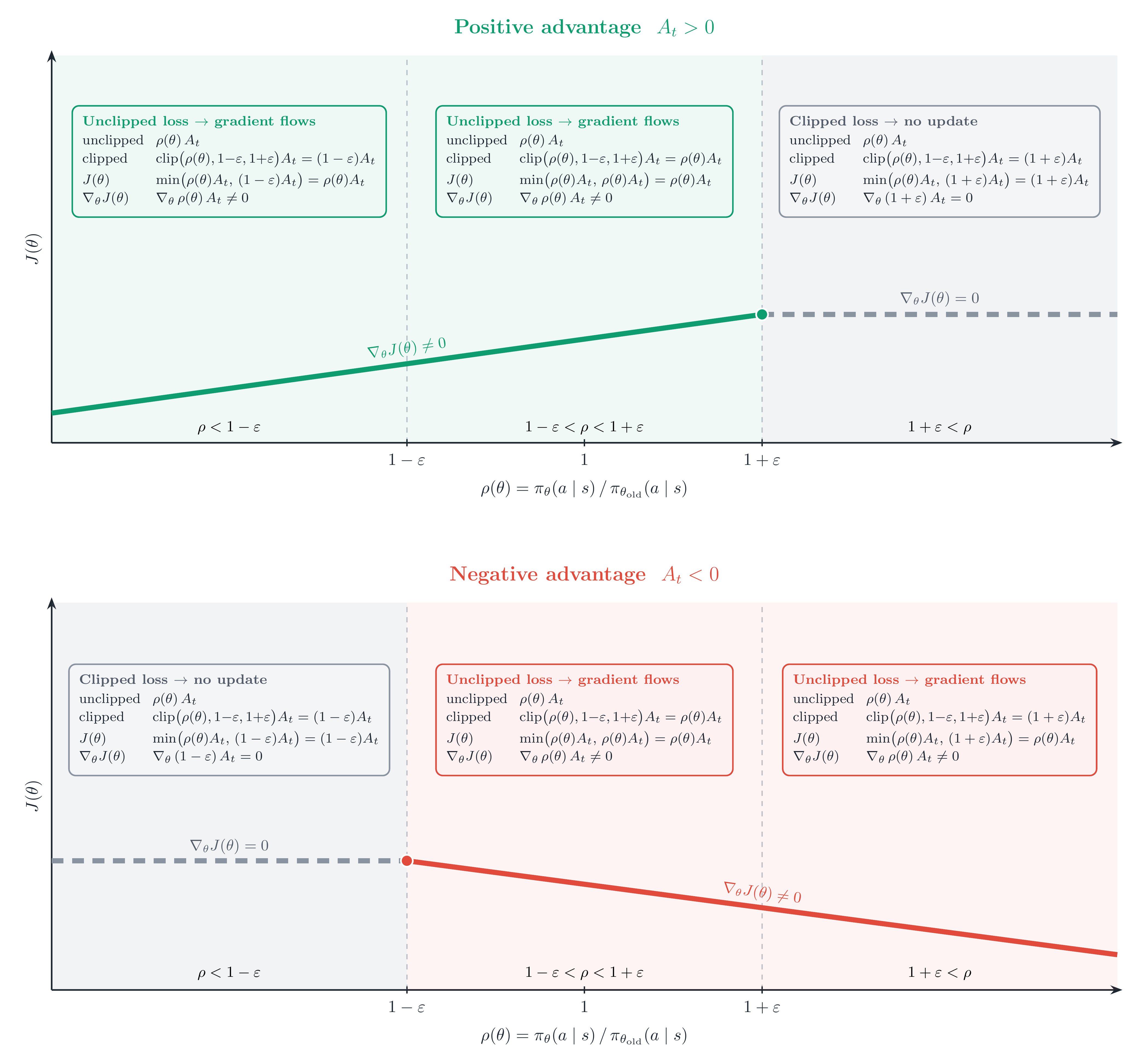
New figure added to Chapter 6 (PR #462, zafstojano)

What comes next?

Introduction & Training Overview – Chapters 1-3
IFT, Reward Models, Rejection Sampling – Chapters 4, 5, 9
RL Theory – Chapter 6 (Part 1)
RL Implementation & Practice – Chapter 6 (Part 2)
Reasoning – Chapter 7
Direct Alignment Algorithms – Chapter 8
Synthetic Data – Chapter 12
Preferences & Preference Data – Chapters 10/11
… shorter lectures on the advanced topics!

Thanks for watching

Questions, comments, and future Q&A prompts:

Course: rlhfbook.com/course
Discord: discord.gg/yz5AwK4gBR
GitHub: github.com/natolambert/rlhf-book
Newsletter: interconnects.ai
Contact: [email protected]

Built withnatolambert/colloquium

References

Lu, K., and Thinking Machines Lab. “On-Policy Distillation.” Thinking Machines Lab: Connectionism, 2025. [link]

Schulman, J.. “Approximating KL Divergence.” 2020.