Chapter Contents

Direct Alignment Algorithms

Direct Alignment Algorithms (DAAs) allow one to update models to solve the same RLHF objective without ever training an intermediate reward model or using reinforcement learning optimizers. The most prominent DAA and one that catalyzed an entire academic movement of aligning language models is Direct Preference Optimization (DPO) [1]. At its core, DPO is using gradient ascent to solve the same constrained RLHF objective. Since its release in May of 2023, after a brief delay where the community figured out the right data and hyperparameters to use DPO with (specifically, surprisingly low learning rates), many popular models have used DPO or its variants, from Zephyr-\(\beta\) kickstarting it in October of 2024 [2], Llama 3 Instruct [3], Tülu 2 [4] and 3 [5], Nemotron 4 340B [6], and others. Technically, Sequence Likelihood Calibration (SLiC-HF) was released first [7], but it did not catch on due to a combination of luck and effectiveness.

The most impactful part of DPO and DAAs is lowering the barrier of entry to experimenting with language model post-training.

Direct Preference Optimization (DPO)

Here we explain intuitions for how it works and re-derive the core equations fully.

How DPO Works

DPO at a surface level is directly optimizing a policy to solve the RLHF objective. The loss function for this, which we will revisit below in the derivations, is a pairwise relationship of log-probabilities. The loss function derived from a Bradley-Terry reward model follows:

\[ \mathcal{L}_{\text{DPO}}(\pi_\theta; \pi_{\text{ref}}) = -\mathbb{E}_{(x, y_c, y_r) \sim \mathcal{D}}\left[ \log \sigma\left( \beta \log \frac{\pi_{\theta}(y_c \mid x)}{\pi_{\text{ref}}(y_c \mid x)} - \beta \log \frac{\pi_{\theta}(y_r \mid x)}{\pi_{\text{ref}}(y_r \mid x)} \right) \right] \qquad{(1)}\]

This relies on the implicit reward for DPO training that replaces using an external reward model, which is a log-ratio of probabilities:

\[r(x, y) = \beta \log \frac{\pi_r(y \mid x)}{\pi_{\text{ref}}(y \mid x)}\qquad{(2)}\]

This comes from deriving the Bradley-Terry reward with respect to an optimal policy (shown in eq. 16), as shown in TODO BT model. Essentially, the implicit reward model shows “the probability of human preference data in terms of the optimal policy rather than the reward model.”

Let us consider the loss shown in eq. 1. The learning process is decreasing the loss. Here, the loss will be lower when the log-ratio of the chosen response is bigger than the log-ratio of the rejected response (normalized by the reference model). In practice, this is a sum of log-probabilities of the model across the sequence of tokens in the data presented. Hence, DPO is increasing the delta in probabilities between the chosen and rejected responses.

With the reward in eq. 2, we can write the gradient of the loss to further interpret what is going on:

\[\nabla_{\theta}\mathcal{L}_{\text{DPO}}(\pi_{\theta}; \pi_{\text{ref}}) = -\beta \mathbb{E}_{(x, y_c, y_r)\sim \mathcal{D}}\left[ \sigma\left(r_{\theta}(x, y_r) - r_{\theta}(x, y_c)\right) \left(\nabla_{\theta}\log \pi(y_c \mid x) - \nabla_{\theta}\log \pi(y_r \mid x)\right) \right] \qquad{(3)}\]

Here, the gradient solves the above objective by doing the following:

• The first term within the sigmoid function, \(\sigma(\cdot)\), creates a weight of the parameter update from 0 to 1 that is higher when the reward estimate is incorrect. When the rejected sample is preferred over the chosen, the weight update should be larger!
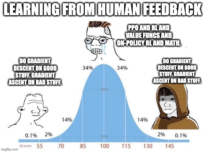
• Second, the terms in the inner brackets \([\cdot]\) increases the likelihood of the chosen response \(y_c\) and decreases the likelihood of the rejected \(y_r\).
• These terms are weighted by \(\beta\), which controls how the update balances ordering the completions correctly relative to the KL distance.

The core intuition is that DPO is “fitting an implicit reward model whose corresponding optimal policy can be extracted in a closed form” (thanks to gradient ascent and our ML tools). What is often misunderstood is that DPO is learning a reward model at its core, hence the subtitle of the paper Your Language Model is Secretly a Reward Model. It is easy to confuse this with the DPO objective training a policy directly, hence studying the derivations below are good for a complete understanding.

With the implicit reward model learning, DPO is generating an optimal solution to the RLHF objective given the data in the dataset and the specific KL constraint in the objective \(\beta\). Here, DPO solves for the exact policy given a specific KL distance because the generations are not online as in policy gradient algorithms – a core difference from the RL methods for preference tuning. In many ways, this makes the \(\beta\) value easier to tune with DPO relative to online RL methods, but crucially and intuitively the optimal value depends on the model being trained and the data training it.

At each batch of preference data, composed of many pairs of completions \(y_{chosen} \succ y_{rejected}\), DPO takes gradient steps directly towards the optimal solution. It is far simpler than policy gradient methods.

DPO Derivation

The DPO derivation takes two primary parts. First, the authors show the form of the policy that optimally solved the RLHF objective used throughout this book. Next, they show how to arrive at that solution from pairwise preference data (i.e. a Bradley Terry model).

1. Deriving the Optimal RLHF Solution

To start, we should consider the RLHF optimization objective once again, here indicating we wish to maximize this quantity:

\[ \max_{\pi} \mathbb{E}_{\tau \sim \pi} \left[r_\theta(s_t, a_t)\right] - \beta \mathcal{D}_{KL}(\pi^{\text{RL}}(\cdot|s_t) \| \pi^{\text{ref}}(\cdot|s_t)).\qquad{(4)}\]

First, let us expand the definition of KL-divergence,

\[\max_{\pi} \mathbb{E}_{x \sim \mathcal{D}}\mathbb{E}_{y \sim \pi(y|x)}\left[r(x,y)-\beta\log\frac{\pi(y|x)}{\pi_{\text{ref}}(y|x)}\right] \qquad{(5)}\]

Next, pull the negative sign out of the difference in brackets. To do this, split it into two terms:

\[ = \max_{\pi}\left(\mathbb{E}_{x \sim \mathcal{D}}\mathbb{E}_{y \sim \pi(y|x)}[r(x,y)] - \beta\,\mathbb{E}_{x \sim \mathcal{D}}\mathbb{E}_{y \sim \pi(y|x)}\left[\log\frac{\pi(y|x)}{\pi_{\text{ref}}(y|x)}\right]\right) \qquad{(6)}\]

Then, remove the factor of \(-1\) and \(\beta\),

\[ = \min_{\pi}\left(-\mathbb{E}_{x \sim \mathcal{D}}\mathbb{E}_{y \sim \pi(y|x)}[r(x,y)] + \beta\,\mathbb{E}_{x \sim \mathcal{D}}\mathbb{E}_{y \sim \pi(y|x)}\left[\log\frac{\pi(y|x)}{\pi_{\mathrm{ref}}(y|x)}\right]\right) \qquad{(7)}\]

Divide by \(\beta\) and recombine:

\[ = \min_{\pi}\left(\mathbb{E}_{x \sim \mathcal{D}}\mathbb{E}_{y \sim \pi(y|x)}\left[ \log\frac{\pi(y|x)}{\pi_{\text{ref}}(y|x)} - \frac{1}{\beta}r(x,y) \right]\right) \qquad{(8)}\]

Next, we must introduce a partition function, \(Z(x)\):

\[ Z(x) = \sum_y \pi_{\text{ref}}(y|x)\exp\left(\frac{1}{\beta}r(x,y)\right) \qquad{(9)}\]

The partition function acts as a normalization factor over the reference policy, summing over all possible responses \(y\) to a prompt \(x\). With this substituted in, we obtain our intermediate transformation:

\[ \min_{\pi}\mathbb{E}_{x\sim\mathcal{D}}\mathbb{E}_{y\sim\pi(y|x)}\left[\log\frac{\pi(y|x)}{\frac{1}{Z(x)}\pi_{\text{ref}}(y|x)\exp\left(\frac{1}{\beta}r(x,y)\right)} - \log Z(x)\right] \qquad{(10)}\]

To see how this is obtained, consider the internal part of the optimization in brackets of eq. 8:

\[ \log\frac{\pi(y|x)}{\pi_{\text{ref}}(y|x)} - \frac{1}{\beta}r(x,y) \qquad{(11)}\]

Then, add \(\log Z(x) - \log Z(x)\) to both sides:

\[ = \log\frac{\pi(y|x)}{\pi_{\text{ref}}(y|x)} - \frac{1}{\beta}r(x,y) + \log Z(x) - \log Z(x) \qquad{(12)}\]

Then, we group the terms:

\[ = \left( \log \frac{\pi(y|x)}{\pi_{\text{ref}}(y|x)} + \log Z(x) \right) - \log Z(x) - \frac{1}{\beta}r(x,y) \qquad{(13)}\]

With \(\log(x) + \log(y) = \log(x\cdot y)\) (and moving \(Z\) to the denominator), we get:

\[ = \log \frac{\pi(y|x)}{\frac{1}{Z(x)}\pi_{\text{ref}}(y|x)}- \log Z(x) - \frac{1}{\beta}r(x,y) \qquad{(14)}\]

Next, we expand \(\frac{1}{\beta}r(x,y)\) to \(\log \exp \frac{1}{\beta}r(x,y)\) and do the same operation to get eq. 10. With this optimization form, we need to actually solve for the optimal policy \(\pi^*\). To do so, let us consider the above optimization as a KL distance:

\[ \min_{\pi}\mathbb{E}_{x\sim\mathcal{D}}\left[\mathbb{D}_\text{KL} \left(\pi(y|x)||\frac{1}{Z(x)}\pi_{\text{ref}}(y|x)\exp\left(\frac{1}{\beta}r(x,y)\right) \right) - \log Z(x)\right] \qquad{(15)}\]

Since the partition function \(Z(x)\) does not depend on the final answer, we can ignore it. This leaves us with just the KL distance between our policy we are learning and a form relating the partition, \(\beta\), reward, and reference policy. The Gibb’s inequality tells this is minimized at a distance of 0, only when the two quantities are equal! Hence, we get an optimal policy:

\[ \pi^*(y|x) = \pi(y|x) = \frac{1}{Z(x)}\pi_{\text{ref}}(y|x)\exp\left(\frac{1}{\beta}r(x,y)\right) \qquad{(16)}\]

2. Deriving DPO Objective for Bradley Terry Models

To start, recall from Chapter 7 on Reward Modeling and Chapter 6 on Preference Data that a Bradley-Terry model of human preferences is formed as:

\[p^*(y_1 \succ y_2 \mid x) = \frac{\exp\left(r^*(y_1 \mid x)\right)}{\exp\left(r^*(x,y_1)\right) + \exp\left(r^*(x, y_2)\right)} \qquad{(17)}\]

By manipulating eq. 16 by taking the logarithm of both sides and performing some algebra, one can obtain the DPO reward as follows:

\[r^*(x, y) = \beta \log \frac{\pi^*(y \mid x)}{\pi_{\text{ref}}(y \mid x)} + \beta \log Z(x)\qquad{(18)}\]

We then can substitute the reward into the Bradley-Terry equation shown in eq. 17 to obtain:

\[p^*(y_1 \succ y_2 \mid x) = \frac{\exp\left(\beta \log \frac{\pi^*(y_1 \mid x)}{\pi_{\text{ref}}(y_1 \mid x)} + \beta \log Z(x)\right)} {\exp\left(\beta \log \frac{\pi^*(y_1 \mid x)}{\pi_{\text{ref}}(y_1 \mid x)} + \beta \log Z(x)\right) + \exp\left(\beta \log \frac{\pi^*(y_2 \mid x)}{\pi_{\text{ref}}(y_2 \mid x)} + \beta \log Z(x)\right)} \qquad{(19)}\]

By decomposing the exponential expressions from \(e^{a+b}\) to \(e^a e^b\) and then cancelling out the terms \(e^{\log(Z(x))}\), this simplifies to:

\[p^*(y_1 \succ y_2 \mid x) = \frac{\exp\left(\beta \log \frac{\pi^*(y_1 \mid x)}{\pi_{\text{ref}}(y_1 \mid x)}\right)} {\exp\left(\beta \log \frac{\pi^*(y_1 \mid x)}{\pi_{\text{ref}}(y_1 \mid x)}\right) + \exp\left(\beta \log \frac{\pi^*(y_2 \mid x)}{\pi_{\text{ref}}(y_2 \mid x)}\right)} \qquad{(20)}\]

Then, multiple the numerator and denominator by \(\exp\left(-\beta \log \frac{\pi^*(y_1 \mid x)}{\pi_{\text{ref}}(y_1 \mid x)}\right)\) to obtain:

\[p^*(y_1 \succ y_2 \mid x) = \frac{1}{1 + \exp\left(\beta \log \frac{\pi^*(y_2 \mid x)}{\pi_{\text{ref}}(y_2 \mid x)} - \beta \log \frac{\pi^*(y_1 \mid x)}{\pi_{\text{ref}}(y_1 \mid x)}\right)} \qquad{(21)}\]

Finally, with the definition of a sigmoid function as \(\sigma(x) = \frac{1}{1+e^{-x}}\), we obtain:

\[p^*(y_1 \succ y_2 \mid x) = \sigma\left(\beta \log \frac{\pi^*(y_1 \mid x)}{\pi_{\text{ref}}(y_1 \mid x)} - \beta \log \frac{\pi^*(y_2 \mid x)}{\pi_{\text{ref}}(y_2 \mid x)}\right) \qquad{(22)}\]

This is the loss function for DPO, as shown in eq. 1. The DPO paper has an additional derivation for the objective under a Plackett-Luce Model, which is far less used in practice [1].

3. Deriving the Bradley Terry DPO Gradient

We used the DPO gradient shown in eq. 3 to explain intuitions for how the model learns. To derive this, we must take the gradient of eq. 22 with respect to the model parameters.

\[\nabla_{\theta}\mathcal{L}_{\text{DPO}}(\pi_{\theta}; \pi_{\text{ref}}) = -\nabla_{\theta}\mathbb{E}_{(x,y_c,y_r)\sim\mathcal{D}}\left[ \log \sigma\left(\beta \log \frac{\pi_{\theta}(y_c|x)}{\pi_{\text{ref}}(y_c|x)} - \beta \log \frac{\pi_{\theta}(y_r|x)}{\pi_{\text{ref}}(y_r|x)}\right)\right] \qquad{(23)}\]

To start, this can be rewritten. We know that the derivative of a sigmoid function \(\frac{d}{dx} \sigma(x) = \sigma(x)(1-\sigma(x))\), the derivative of logarithm \(\frac{d}{dx} \log x = \frac{1}{x}\), and properties of sigmoid \(\sigma(-x)=1-\sigma(x)\), so we can reformat the above equation.

First, define the expression inside the sigmoid as \(u=\beta \log \frac{\pi_{\theta}(y_c|x)}{\pi_{\text{ref}}(y_c|x)} - \beta \log \frac{\pi_{\theta}(y_r|x)}{\pi_{\text{ref}}(y_r|x)}\). Then, we have

\[\nabla_{\theta}\mathcal{L}_{\text{DPO}}(\pi_{\theta};\pi_{\text{ref}}) = -\mathbb{E}_{(x, y_c, y_r)\sim \mathcal{D}}\left[\frac{\sigma'(u)}{\sigma(u)}\nabla_{\theta}u\right] \qquad{(24)}\]

Expanding this and using the above expressions for sigmoid and logarithms results in the gradient introduced earlier:

\[ -\mathbb{E}_{(x,y_c,y_r)\sim\mathcal{D}}\left[\beta\sigma\left(\beta\log\frac{\pi_{\theta}(y_r|x)}{\pi_{\text{ref}}(y_r|x)} - \beta\log\frac{\pi_{\theta}(y_c|x)}{\pi_{\text{ref}}(y_c|x)}\right)\left[\nabla_{\theta}\log\pi(y_c|x)-\nabla_{\theta}\log\pi(y_r|x)\right]\right] \qquad{(25)}\]

Numerical Concerns, Weaknesses, and Alternatives

Many variants of the DPO algorithm have been proposed to address weaknesses of DPO. For example, without rollouts where a reward model can rate generations, DPO treats every pair of preference data with equal weight. In reality, as seen in Chapter 6 on Preference Data, there are many ways of capturing preference data with a richer label than binary. Multiple algorithms have been proposed to re-balance the optimization away from treating each pair equally.

• REgression to RElative REward Based RL (REBEL) adds signal from a reward model, as a margin between chosen and rejected responses, rather than solely the pairwise preference data to more accurately solve the RLHF problem [8].
• Conservative DPO (cDPO) and Identity Preference Optimization (IPO) address the overfitting by assuming noise in the preference data. cDPO assumes N percent of the data is incorrectly labelled [1] and IPO changes the optimization to soften probability of preference rather than optimize directly from a label [9]. Practically, IPO changes the preference probability to a nonlinear function, moving away from the Bradley-Terry assumption, with \(\Psi(q) = \log\left(\frac{q}{1-q}\right)\).
• DPO with an offset (ODPO) “requires the difference between the likelihood of the preferred and dispreferred response to be greater than an offset value” [10] – do not treat every data pair equally, but this can come at the cost of a more difficult labeling environment.

Some variants to DPO attempt to either improve the learning signal by making small changes to the loss or make the application more efficient by reducing memory usage.

• Odds Ratio Policy Optimization (ORPO) directly updates the policy model with a pull towards the chosen response, similar to the instruction finetuning loss, with a small penalty on the chosen response [11]. This change of loss function removes the need for a reference model, simplifying the setup. The best way to view ORPO is DPO inspired, rather than a DPO derivative.
• Simple Preference Optimization SimPO makes a minor change to the DPO optimization, by averaging the log-probabilities rather than summing them (SimPO) or adding length normalization, to improve performance [12].

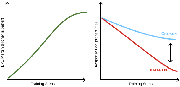
One of the core issues apparent in DPO is that the optimization drives only to increase the margin between the probability of the chosen and rejected responses. Numerically, the model reduces the probabiltiy of both the chosen and rejected responses, but the rejected response is reduced by a greater extent as shown in fig. 2. Intuitively, it is not clear how this generalizes, but work has posited that it increases the probability of unaddressed for behaviors [13] [14]. Simple methods, such as Cal-DPO [15], adjust the optimization so that this preference displacement does not occur. In practice, the exact impact of this is not well known, but points are a potential reason why online methods can outperform vanilla DPO.

The largest other reason that is posited for DPO-like methods to have a lower ceiling on performance than online (RL based) RLHF methods is that the training signal comes from completions from previous or other models. Online variants that sample generations from the model, e.g. Online DPO [16], even with regular reward model relabelling of newly created creations Discriminator-Guided DPO (D2PO) [17], alleviate these by generating new completions for the prompt and incorporating a preference signal at training time.

There is a long list of other DAA variants, such as Direct Nash Optimization (DNO) [18] or Binary Classifier Optimization (BCO) [19], but the choice of algorithm is far less important than the initial model and the data used [5] [20] [21].

Implementation Considerations

DAAs such as DPO are implemented very differently than policy gradient optimizers. The DPO loss, taken from the original implementation, largely can be summarized as follows [1]:

pi_logratios = policy_chosen_logps - policy_rejected_logps
ref_logratios = reference_chosen_logps - reference_rejected_logps

logits = pi_logratios - ref_logratios  # also known as h_{\pi_\theta}^{y_w,y_l}

losses = -F.logsigmoid(beta * logits)

chosen_rewards = beta * (policy_chosen_logps - reference_chosen_logps).detach()
rejected_rewards = beta * (policy_rejected_logps - reference_rejected_logps).detach()

This can be used in standard language model training stacks as this information is already collated during the forward pass of a model (with the addition of a reference model).

In most ways, this is simpler and an quality of life improvement, but also they offer a different set of considerations.

1. KL distance is static: In DPO and other algorithms, the KL distance is set explicitly by the \(\beta\) parameter that balances the distance penalty to the optimization. This is due to the fact that DPO takes gradient steps towards the optimal solution to the RLHF objective given the data – it steps exactly to the solution set by the \(\beta\) term. On the other hand, RL based optimizers take steps based on the batch and recent data.
2. Caching log-probabilities: Simple implementations of DPO do the forward passes for the policy model and reference models at the same time for conveniences with respect to the loss function. Though, this doubles the memory used and results in increased GPU usage. To avoid this, one can compute the log-probabilities of the reference model over the training dataset first, then reference it when computing the loss and updating the parameters per batch, reducing the peak memory usage by 50%.

DAAs vs. RL: Online vs. Offline Data

Broadly, the argument boils down to one question: Do we need the inner workings of reinforcement learning, with value functions, policy gradients, and all, to align language models with RLHF? This, like most questions phrased this way, is overly simplistic. Of course, both methods are well-established, but it is important to illustrate where the fundamental differences and performance manifolds lie.

Multiple reports have concluded that policy-gradient based and RL methods outperform DPO and its variants. The arguments take different forms, from training models with different algorithms but controlled data[22] [23] or studying the role of on-policy data within the RL optimization loop [24]. In all of these cases, DPO algorithms are a hair behind.

Even with this performance delta, DAA are still used extensively in leading models due to its simplicity. DAAs provide a controlled environment where iterations on training data and other configurations can be made rapidly, and given that data is often far more important than algorithms, using DPO can be fine.

With the emergence of reasoning models that are primarily trained with RL, further investment will return to using RL for preference-tuning, which in the long-term will improve the robustness of RL infrastructure and cement this margin between DAAs and RL for optimizing from human feedback.

Bibliography