Rejection Sampling
Rejection Sampling (RS) is a popular and simple baseline for performing preference fine-tuning. Rejection sampling operates by curating new candidate instructions, filtering them based on a trained reward model, and then fine-tuning the original model only on the top completions.
The name originates from computational statistics [1], where one wishes to sample from a complex distribution, but does not have a direct method to do so. To alleviate this, one samples from a simpler to model distribution and uses a heuristic to check if the sample is permissible. With language models, the target distribution is high-quality answers to instructions, the filter is a reward model, and the sampling distribution is the current model.
Related works
Many prominent RLHF and preference fine-tuning papers have used rejection sampling as a baseling, but a canonical implementation and documentation does not exist
WebGPT [2], Anthropic’s Helpful and Harmless agent[3], OpenAI’s popular paper on process reward models [4], Llama 2 Chat models [5], and other seminal works all use this baseline.
Training Process
A visual overview of the rejection sampling process is included
below. 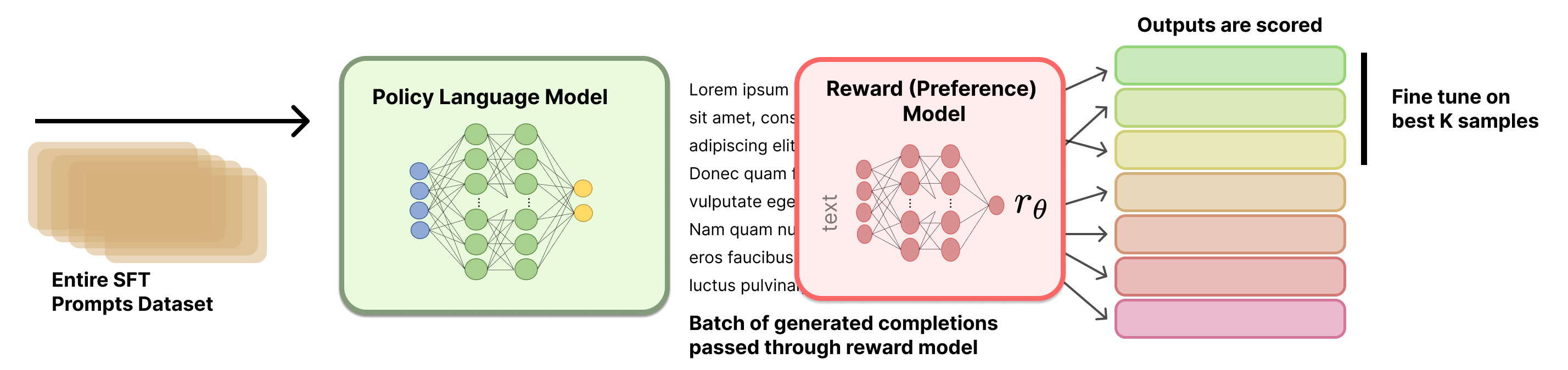
Generating Completions
Let’s define a set of \(M\) prompts as a vector:
\[X = [x_1, x_2, ..., x_M]\]
These prompts can come from many sources, but most popularly they come from the instruction training set.
For each prompt \(x_i\), we generate \(N\) completions. We can represent this as a matrix:
\[Y = \begin{bmatrix} y_{1,1} & y_{1,2} & \cdots & y_{1,N} \\ y_{2,1} & y_{2,2} & \cdots & y_{2,N} \\ \vdots & \vdots & \ddots & \vdots \\ y_{M,1} & y_{M,2} & \cdots & y_{M,N} \end{bmatrix}\]
where \(y_{i,j}\) represents the \(j\)-th completion for the \(i\)-th prompt. Now, we pass all of these prompt-completion pairs through a reward model, to get a matrix of rewards. We’ll represent the rewards as a matrix R:
\[R = \begin{bmatrix} r_{1,1} & r_{1,2} & \cdots & r_{1,N} \\ r_{2,1} & r_{2,2} & \cdots & r_{2,N} \\ \vdots & \vdots & \ddots & \vdots \\ r_{M,1} & r_{M,2} & \cdots & r_{M,N} \end{bmatrix}\]
Each reward \(r_{i,j}\) is computed by passing the completion \(y_{i,j}\) and its corresponding prompt \(x_i\) through a reward model \(\mathcal{R}\):
\[r_{i,j} = \mathcal{R}(y_{i,j}|x_i)\]
Selecting Top-N Completions
There are multiple methods to select the top completions to train on.
To formalize the process of selecting the best completions based on our reward matrix, we can define a selection function \(S\) that operates on the reward matrix \(R\).
Top Per Prompt
The first potential selection function takes the max per prompt.
\[S(R) = [\arg\max_{j} r_{1,j}, \arg\max_{j} r_{2,j}, ..., \arg\max_{j} r_{M,j}]\]
This function \(S\) returns a vector of indices, where each index corresponds to the column with the maximum reward for each row in \(R\). We can then use these indices to select our chosen completions:
\[Y_{chosen} = [y_{1,S(R)_1}, y_{2,S(R)_2}, ..., y_{M,S(R)_M}]\]
Top Overall Prompts
Alternatively, we can select the top K prompt-completion pairs from the entire set. First, let’s flatten our reward matrix R into a single vector:
\[R_{flat} = [r_{1,1}, r_{1,2}, ..., r_{1,N}, r_{2,1}, r_{2,2}, ..., r_{2,N}, ..., r_{M,1}, r_{M,2}, ..., r_{M,N}]\]
This \(R_{flat}\) vector has length \(M \times N\), where M is the number of prompts and N is the number of completions per prompt.
Now, we can define a selection function \(S_K\) that selects the indices of the K highest values in \(R_{flat}\):
\[S_K(R_{flat}) = \text{argsort}(R_{flat})[-K:]\]
where \(\text{argsort}\) returns the indices that would sort the array in ascending order, and we take the last K indices to get the K highest values.
To get our selected completions, we need to map these flattened indices back to our original completion matrix Y. We simply index the \(R_{flat}\) vector to get our completions.
Selection Example
Consider the case where we have the following situation, with 5 prompts and 4 completions. We will show two ways of selecting the completions based on reward.
\[R = \begin{bmatrix} 0.7 & 0.3 & 0.5 & 0.2 \\ 0.4 & 0.8 & 0.6 & 0.5 \\ 0.9 & 0.3 & 0.4 & 0.7 \\ 0.2 & 0.5 & 0.8 & 0.6 \\ 0.5 & 0.4 & 0.3 & 0.6 \end{bmatrix}\]
First, per prompt. Intuitively, we can highlight the reward matrix as follows:
\[R = \begin{bmatrix} \textbf{0.7} & 0.3 & 0.5 & 0.2 \\ 0.4 & \textbf{0.8} & 0.6 & 0.5 \\ \textbf{0.9} & 0.3 & 0.4 & 0.7 \\ 0.2 & 0.5 & \textbf{0.8} & 0.6 \\ 0.5 & 0.4 & 0.3 & \textbf{0.6} \end{bmatrix}\]
Using the argmax method, we select the best completion for each prompt:
\[S(R) = [\arg\max_{j} r_{i,j} \text{ for } i \in [1,4]]\]
\[S(R) = [1, 2, 1, 3, 4]\]
This means we would select:
- For prompt 1: completion 1 (reward 0.7)
- For prompt 2: completion 2 (reward 0.8)
- For prompt 3: completion 1 (reward 0.9)
- For prompt 4: completion 3 (reward 0.8)
- For prompt 5: completion 4 (reward 0.6)
Now, best overall. Let’s highlight the top 5 overall completion pairs.
\[R = \begin{bmatrix} \textbf{0.7} & 0.3 & 0.5 & 0.2 \\ 0.4 & \textbf{0.8} & 0.6 & 0.5 \\ \textbf{0.9} & 0.3 & 0.4 & \textbf{0.7} \\ 0.2 & 0.5 & \textbf{0.8} & 0.6 \\ 0.5 & 0.4 & 0.3 & 0.6 \end{bmatrix}\]
First, we flatten the reward matrix:
\[R_{flat} = [0.7, 0.3, 0.5, 0.2, 0.4, 0.8, 0.6, 0.5, 0.9, 0.3, 0.4, 0.7, 0.2, 0.5, 0.8, 0.6, 0.5, 0.4, 0.3, 0.6]\]
Now, we select the indices of the 5 highest values: \[S_5(R_{flat}) = [8, 5, 14, 0, 19]\]
Mapping these back to our original matrix:
- Index 8 → prompt 3, completion 1 (reward 0.9)
- Index 5 → prompt 2, completion 2 (reward 0.8)
- Index 14 → prompt 4, completion 3 (reward 0.8)
- Index 0 → prompt 1, completion 1 (reward 0.7)
- Index 19 → prompt 3, completion 4 (reward 0.7)
Implementation Example
Here is a code snippet showing how the selection methods could be implemented.
import numpy as np

x = np.random.randint(10, size=10)
print(f"{x=}")
sorted_indices = np.argsort(x)
x_sorted = x[sorted_indices]
print(f"{x_sorted=}")

# first way to recover the original array
i_rev = np.zeros(10, dtype=int)
i_rev[sorted_indices] = np.arange(10)
np.allclose(x, x_sorted[i_rev])

# second way to recover the original array
np.allclose(x, x_sorted[np.argsort(sorted_indices)])
Fine-tuning
With the selected completions, you then perform standard instruction fine-tuning on the current rendition of the model. More details can be found in the chapter on instruction tuning.
Details
Implementation details for rejection sampling are relatively sparse. The core hyperparameters for performing this training are very intuitive:
- Sampling parameters: Rejection sampling is directly dependent on the completions received from the model. Common settings for RS include tempetures above zero, e.g. between 0.7 and 1.0, with other modifications to paramters such as top-p or top-k sampling.
- Completions per prompt: Successful implementations of rejection sampling have included 10 to 30 or more completions for each prompt. Using too few completions will make training biased and or noisy.
- Instruction tuning details: No clear training details for the instruction tuning during RS have been released. It is likely that they use slightly different settings than the initial instruction tuning phase of the model.
- Hetergenous model generations: Some implementations of rejection sampling include generations from multiple models rather than just the current model that is going to be trained. Best practices on how to do this are not established.
- Reward model training: The reward model used will heavily impact the final result. For more resources on reward model training, see the relevant chapter.
Implementation Tricks
- When doing batch reward model inference, you can sort the tokenized completions by length so that the batches are of similar lengths. This eliminates the need to run inference on as many padding tokens and will improve throughput in exchange for minor implementation complexity.
Related: Best-of-N Sampling
Best-of-N (BoN) sampling is often included as a baseline relative to RLHF methods. It is important to remember that BoN does not modify the underlying model, but is a sampling technique. For this matter, comparisons for BoN sampling to online training methods, such as PPO, is still valid in some contexts. For example, you can still measure the KL distance when running BoN sampling relative to any other policy.
Here, we will show that when using simple BoN sampling over one prompt, both selection criteria shown above are equivalent.
Let R be a reward vector for our single prompt with N completions:
\[R = [r_1, r_2, ..., r_N]\]
Where \(r_j\) represents the reward for the j-th completion.
Using the argmax method, we select the best completion for the prompt: \[S(R) = \arg\max_{j \in [1,N]} r_j\]
Using the Top-K method is normally done with Top-1, reducing to the same method.